Data Science: Interpolate Air Quality Measurements with Python

Update

• 2022-09-11 Tutorial has been updated to the new version of pyinterpolate. New figures and text corrections.

How do we measure air quality? The most popular are stationary sensors that detect the amount of toxic compounds in the air. Each sensor’s readings may be described by [timestamp, latitude, longitude, value]. Sensors do not cover a big area. We can’t expect observations to be taken at a regular grid, which is easy to interpolate. The final image from the raw data source may look like this one:

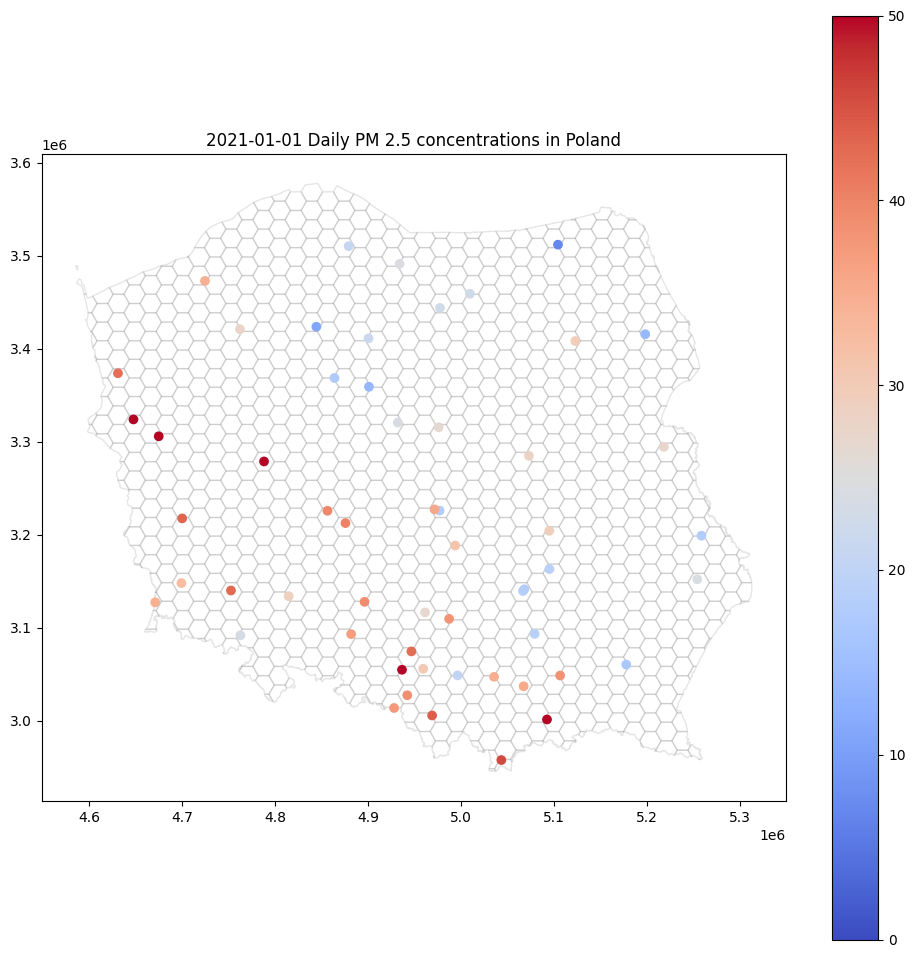
This type of point map may be helpful for experts, but the general public will be bored, or much worse – confused – by this kind of visualization. There are so many white areas! Fortunately, we can interpolate air pollution in every hex within this map. We are going to learn how to do it step-by-step. We will use the Ordinary Kriging method implemented in pyinterpolate package.

Data

We are going to use two datasets. One represents point measurements of PM2.5 concentrations, and another is a hex-grid over which we will interpolate PM2.5 concentrations. You should be able to follow each step in this article with your data. Just have in mind those constraints:

• both datasets should have the same projection,
• points should be within the hexgrid (or other blocks / MultiPolygon) area.

The PM 2.5 measurements are available here, and you may download the hexgrid here.

Setup

The safest method of setup is to create a conda environment and install the package within it. Pyinterpolate works ith Python 3.7 up to Python 3.10 and within UNIX systems, so if you are a Windows user, you should consider using Windows Subsystem for Linux (WSL).

Let’s start with conda environment preparation:

conda create -n [NAME OF YOUR ENV]

We name the environment as spatial-interpolate, but you may consider your own name:

conda create -n spatial-interpolate

Next, activate the environment:

conda activate spatial-interpolate

Then install core packages, I assume you use Python 3.7+ as your base version (Python 3.7, 3.8, 3.9, or 3.10):

(spatial-interpolate) conda install -c conda-forge pip notebook

And install pyinterpolate with pip:

(spatial-interpolate) pip install pyinterpolate

Sometimes you may get an error related to a missing package named libspatialindex_c.so. To install it on Linux, write in the terminal:

sudo apt install libspatialindex-dev

And to install it on macOS, use this command in the terminal:

brew install spatialindex

At this point, we should be able to move forward. But, if you encounter any problems, don’t hesitate to ask for help here.

Read Data

Our task is to transform point observations into a country-wide hexgrid. Observations are stored in a csv file. Each column is a timestamp, and rows represent stations. Two additional columns x and y are longitude and latitude of a station. The hexgrid is a shapefile which consists of six different types of files. We need to read only one of those – with .shp prefix – but all others must be placed in the same directory, with the same suffix name. The csv file could be read with pandas. Shapefile must be loaded with geopandas.

We will import all functions and packages in the first cell of a notebook, then we will read files and check how they look inside.

import pandas as pd
import geopandas as gpd
import numpy as np
from pyproj import CRS

from pyinterpolate import build_experimental_variogram, TheoreticalVariogram, kriging

We have imported a lot of stuff here! Let’s check for what are those packages and functions responsible:

• pandas: read csv file,
• geopandas: read shapefile and transform geometries,
• numpy: algebra and matrix operations,
• pyproj.CRS: sets Coordinate Reference System (projection of points),
• build_experimental_variogram(): calculate the error between observations in the function of the distance,
• TheoreticalVariogram: create a model of dissimilarity between samples in the function of the distance,
• kriging(): Interpolate missing values from a set of points and a semivariogram.

Don’t worry if you don’t understand all terms above. We will see what they do in practice in the following steps.

readings = pd.read_csv('pm25_year_2021_daily.csv', index_col='name')
canvas = gpd.read_file('hexgrid.shp')
canvas['points'] = canvas.centroid

Variable readings is a DataFrame with 153 columns from which two columns are spatial coordinates. The rest are a daily average of PM 2.5 concentration. It is a time series, but we are going to select one date for further analysis. Variable canvas represents a set of geometries and their ids. Geometries are stored as hexagonal blocks. We need to create a point grid from those blocks. It is straightforward in GeoPandas. We can use the .centroid attribute to get the centroid of each geometry.

We will limit the number of columns in DataFrame to ['01.01.2021', 'x', 'y'] and rename the first column to pm2.5:

df = readings[['01.01.2021', 'x', 'y']]
df.columns = ['pm2.5', 'x', 'y']

Transform DataFrame into GeoDataFrame (Optional)

We can transform our DataFrame into GeoDataFrame to have the ability to show data as a map. There are two basic steps to do it correctly. First, we should prepare Coordinate Reference System (CRS). It is not simple to assign concrete CRS from scratch because it has multiple properties. Let’s take a look at CRS used to work with geographical data over Poland:

<Projected CRS: EPSG:2180>
Name: ETRF2000-PL / CS92
Axis Info [cartesian]:
- x[north]: Northing (metre)
- y[east]: Easting (metre)for the European Petroleum Survey Group
Area of Use:
- name: Poland - onshore and offshore.
- bounds: (14.14, 49.0, 24.15, 55.93)
Coordinate Operation:
- name: Poland CS92
- method: Transverse Mercator
Datum: ETRF2000 Poland
- Ellipsoid: GRS 1980
- Prime Meridian: Greenwich

We are not going to write such long descriptions. Fortunately for us, the European Petroleum Survey Group (EPSG) created a database with numbered indexes that point directly to the most common CRS. We use EPSG:2180 (look into the first row of CRS, and you’ll see it). Python’s pyproj package has a built-in database of EPSG-CRS pairs. We can provide an EPSG number to get specific CRS:

DATA_CRS = CRS.from_epsg('2180')

Bear in mind that we already know CRS/EPSG of a data source. Sometimes it is not so simple with data retrieved from CSV files. You will be forced to dig deeper or try a few projections blindly to get a valid geometry (my first try is usually EPSG 4326 – from GPS coordinates). The next step is to transform our floating-point coordinates into Point() geometry. After this transformation and setting a CRS, we get a GeoDataFrame.

df['geometry'] = gpd.points_from_xy(df['x'], df['y'])
gdf = gpd.GeoDataFrame(df, geometry='geometry', crs=DATA_CRS)

We can show our data on a map! First, we remove NaN rows, and then we will visualize available points over a canvas used for interpolation.

# Remove NaNs

gdf = gdf.dropna()

base = canvas.plot(color='white', edgecolor='black', alpha=0.1, figsize=(12, 12))
gdf.plot(ax=base, column='pm2.5', legend=True, vmin=0, vmax=50, cmap='coolwarm')
base.set_title('2021-01-01 Daily PM 2.5 concentrations in Poland');

Build a variogram model

Before interpolation, we must create the (semi)variogram model. What is it? It is a function that measures dissimilarity between points. Its foundation is an assumption that close points tend to be similar and distant points are usually different. This simple technique is a potent tool for analysis. To make it work, we must set a few constants:

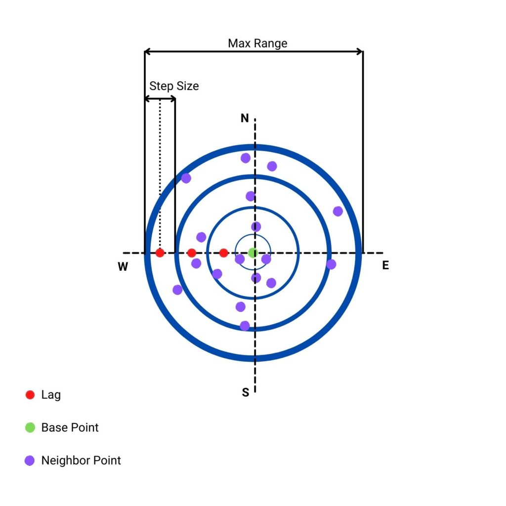
• STEP_SIZE: the distance within points are grouped (binned) together. We start from a distance zero, then 0 + STEP_SIZE from a point and so on. We test the average dissimilarity of a point and its neighbors within the step size i and step size i+1.
• MAX_RANGE: maximum range of analysis. At some range there is no correlation between points and it is a waste of resources to analyze such distant radius from the initial point. MAX_RANGE should be smaller than the maximum distance between points in dataset. Usually it is a half of the maximum distance.

The critical thing to notice is to set STEP_SIZE and MAX_RANGE in the units of data. Sometimes you get coordinates in degrees and sometimes in meters. You should always be aware of this fact. Our projection unit is a meter. We can check that the maximum distance between points could be close to 500 km. Thus, we set our maximum range close to the upper limit, to 400 kilometers.

km_c = 10**3
STEP_SIZE = km_c * 50
MAX_RANGE = km_c * 400

Pyinterpolate operates on numpy arrays. That’s why we must provide only [x, y, pm2.5] as an array of values instead of GeoDataFrame for build_experimental_variogram() function. We use this array along with STEP_SIZE and MAX_RANGE and calculate spatial dissimilarity between points with build_experimental_variogram() function:

arr = gdf[['x', 'y', 'pm2.5']].values

semivar = build_experimental_variogram(input_array=arr, step_size=STEP_SIZE, max_range=MAX_RANGE)

It is an intermediate step. If you print semivar you will see an array with three columns:

array([[0.00000000e+00, 5.05416667e+00, 6.00000000e+01],
       [3.00000000e+04, 5.76951786e+01, 5.60000000e+01],
       [6.00000000e+04, 9.47646939e+01, 9.80000000e+01],
       [9.00000000e+04, 7.46993333e+01, 1.50000000e+02],
       [1.20000000e+05, 7.45332632e+01, 1.90000000e+02],
       [1.50000000e+05, 1.31586140e+02, 2.28000000e+02],
       [1.80000000e+05, 1.24392830e+02, 2.12000000e+02],
       [2.10000000e+05, 1.40270976e+02, 2.46000000e+02],
       [2.40000000e+05, 1.41650229e+02, 2.18000000e+02],
       [2.70000000e+05, 1.42644732e+02, 2.24000000e+02]])

What is the meaning of each column?

• Column 1 is the lag. We test all points within (lag - 0.5 * step size, lag + 0.5 * step size]. (It is done under the hood with function select_values_in_range()).. To make it easier to understand, let’s look into the figure below that shows lags, step size, and max range from the perspective of a single point.

• Column 2 is the semivariance. We can understand this parameter as a measurement of dissimilarity between points within bins given by a lag and a step size. It is averaged value for all points and their neighbors per lag.
• Column 3 is a number of points within a specific distance.

What we have created is the experimental semivariogram. With it, we can create a theoretical model of semivariance. Pyinterpolate has a particular class for semivariogram modeling named TheoreticalVariogram. It takes an array of known points and the experimental semivariogram during initialization. We can model a semivariogram manually, but TheoreticalVariogram class has a method to do it automatically. It is named .autofit(). It returns the best model parameters and an error level (RMSE, Forecast Bias, Mean Absolute Error, or Symmetric Mean Absolute Percentage Error):

ts = TheoreticalVariogram()
ts.autofit(experimental_variogram=semivar, verbose=False)

{'model_type': 'exponential',
 'nugget': 0,
 'sill': 148.20096938775512,
 'rang': 115532.31719150333,
 'fitted_model': array([[5.00000000e+04, 5.20624642e+01],
        [1.00000000e+05, 8.58355732e+01],
        [1.50000000e+05, 1.07744311e+02],
        [2.00000000e+05, 1.21956589e+02],
        [2.50000000e+05, 1.31176145e+02],
        [3.00000000e+05, 1.37156904e+02],
        [3.50000000e+05, 1.41036644e+02]]),
 'rmse': 5.590562271875477,
 'bias': nan,
 'mae': nan,
 'smape': nan}

Another helpful method is .plot(). It draws the experimental points and the theoretical curve, we can check if the semivariogram is valid or wrong and compare how the model behaves at a close distance against long distances.

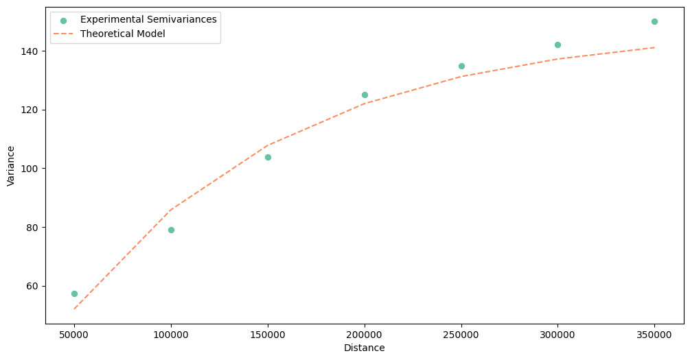
As you see, the dissimilarity increases over distance. Distant points tend to have different PM 2.5 concentrations.

Interpolate Missing Values with Kriging

The last step of our tutorial is interpolation. We use the kriging method. It is a function that predicts values at unknown locations based on the closest neighbors and theoretical semivariance. In practice, it multiplies concentrations of n-closest neighbors by weights related directly to the distance from the predicted location to its neighbor. Pyinterpolate makes this operation extremely simple. We use kriging() function and pass into it five parameters:

1. observations: array with triplets [x, y, value], those are known measurements.
2. theoretical_model: fitted TheoreticalVariogram model.
3. points: a list of points to interpolate values.
4. neighbors_range: a distance within we include neighbors to interpolate a missing value.
5. no_neighbors: the number of neighbors to include in interpolation (if there are more neighbors in the neighbors_range than no_neighbors, then the algorithm takes only the first no_neighbors points based on the sorted distances.

# Predict

pts = list(zip(canvas['points'].x, canvas['points'].y))  # Here we get points from canvas

predicted = kriging(observations=arr,
                    theoretical_model=ts,
                    points=pts,
                    neighbors_range=MAX_RANGE / 2,
                    no_neighbors=8)

Do you remember when we created centroids for our hexagonal canvas? We have named column with these points. Now we use every row of this column and interpolate PM 2.5 concentration for it!

After prediction, we will transform output array into a GeoDataFrame to show results and store them for the future work:

cdf = gpd.GeoDataFrame(data=predicted, columns=['yhat', 'err', 'x', 'y'])
cdf['geometry'] = gpd.points_from_xy(cdf['x'], cdf['y'])
cdf.set_crs(crs=DATA_CRS, inplace=True)

Function get_prediction() is passed in the apply method. It takes three parameters

The kriging() function returns four objects:

1. Estimated value.
2. Error.
3. Longitude.
4. Latitude.

We create GeoDataFrame from those, create geometry (column and attribute) and set CRS. Then, we can visualize the output:.

Below the body of a get_prediction() function, we have a classical operation on DataFrames. Finally, we can show results:

base = canvas.plot(color='white', edgecolor='black', alpha=0.1, figsize=(12, 12))
cdf.plot(ax=base, column='yhat', legend=True, cmap='coolwarm')
base.set_title('Interpolated 2021-01-01 Daily PM 2.5 concentrations in Poland');

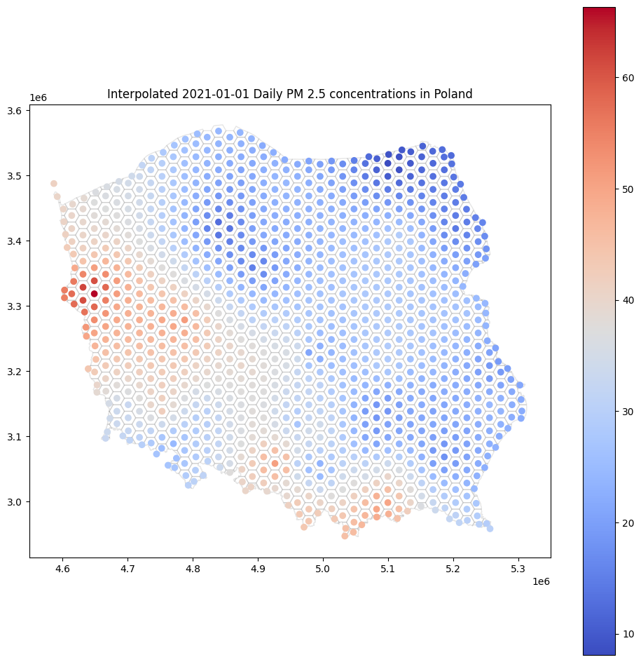
Isn’t it much more interesting than scatterplot?

Additional Reading

1. More about Semivariogram Modeling within pyinterpolate
2. More about Kriging within pyinterpolate
3. Learn about spatial interpolation!

Exercise

1. Try to reproduce this tutorial with other measurements. For example, temperature readings, height above sea level, humidity…