Set this right! – How to prepare recommendation system for the real world

Session-based recommendation engine in Python

Part 4

Introduction

Every model is founded on high-quality data. Assuming a clean and representative dataset, you may start thinking about the model’s hyperparameters. WSKNN recommendation model has multiple settings, and we will test them to see how they affect recommendations. Before we start, you should know that if you use WSKNN package and its internal algorithm, you can change model parameters on the fly, even during the inference! What’s the catch? The model grows very fast because it duplicates data; thus, it is unreliable for enormous datasets.

Here is the list of model parameters in the package wsknn==1.2:

1. The number of recommendations.
2. Sample size.
3. Sampling strategy.
4. Number of neighbors.
5. Weighting function.
6. Ranking strategy.
7. Known items.
8. Required action and its index.
9. Custom weights.
10. Random recommendations.

We will describe each parameter and check how single or multiple parameters can change the model scoring and inference time.

(1) Number of recommendations

Parameter name: number_of_recommendations

Default value: 5

Short description: the number of recommended products

Long description: This parameter doesn’t switch anything within a trained model but affects the number of outputs. We show five recommendations for online shops typically. Sometimes, we need more results. WSKNN returns every recommendation with a weight; thus, we can set this parameter to a large value and cut off low-weighted recommendations. UI/UX design might impose how many recommendations a model returns. This parameter is related to (7) and (10) – those three parameters profoundly affect the output.

(2) Sample size

Parameter name: sample_size

Default value: 1000

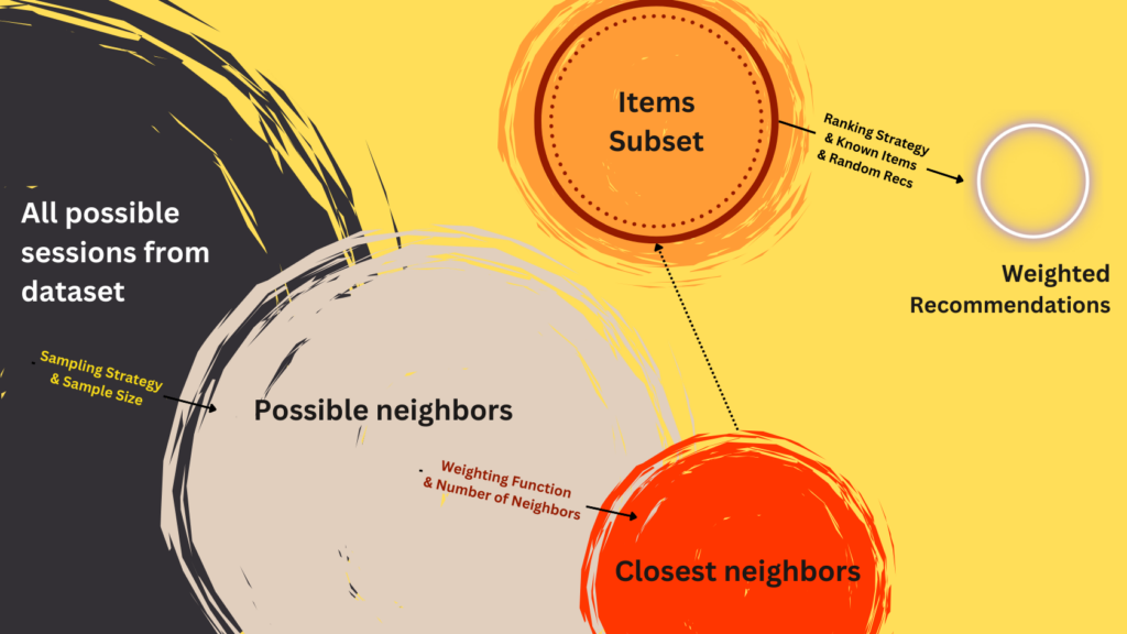
Short description: how many sessions from the model are sampled to make a recommendation, the possible neighbors space

Long description: This is the first parameter that changes the internal workings of the WSKNN architecture. Typically, the model stores billions of sessions. Checking every session’s similarity could be cumbersome. The model makes a recommendation using only a subset of all available sessions. It chooses the subset using the strategy provided by the parameter (3) Sampling Strategy.

(3) Sampling strategy

Parameter name: sampling_strategy

Default value: "common_items"

Short description: initial session-filtering options

Long description: The WSKNN network has thousands of sessions, and it would be unreliable to check the similarity with every session in a set. That’s why we set the sample size (2) and chose a sampling strategy from four options:

• "random": algorithm picks a random subset of sessions. It prevents overfitting and works nicely with the random recommendations parameter (10)
• "recent": algorithm selects the most recent records. Invaluable when data presents cyclic or seasonal patterns, short-lived trends, and anomalies
• "common_items": we want to recommend products that are most frequently grouped within a session
• "weighted_events": we can assign weights to each event; for example, actions like product view, go to checkout, and purchase will have different weights. We use sessions with the highest weights (usually those ending with purchase)

(4) Number of neighbors

Parameter name: number_of_neighbors

Default value: 10

Short description: the number of the closest sessions to choose the items from

Long description: The set of possible neighbors (2, 3) is limited again after session-weighting (5) of the possible neighbors. Why? Because the item space could still be too large to make fast calculations. From these neighbors, we will rank items and make recommendations. The figure below shows the whole process and links parameters to each process step.

(5) Weighting function

Parameter name: weighting_func

Default value: "linear"

Short description: The possible neighbor’s sessions weighting and ranking method

Long description: Using this parameter, we rank the possible neighbors from steps (2, 3) and create the closest neighbors set of the size given in step (4). We have three possible weighting functions, and with every function, we compare the user session for recommendation to the possible neighbors’ sessions. Items ordering is essential!

• "linear": weight is proportional to the position of an item in a possible neighbor session. The newest elements (last on the list) get higher weights.
• "log": works like "linear" but older elements get smaller weights. This function mimics short-term memory, emphasizes the newest elements, and gives larger weights for short-sequence items. 
• "quadratic": similarly to "log" penalizes the oldest elements in sequence more.

We get ranked sessions of the possible neighbors, then sort them and slice them up to the number of the closest neighbors. Those sessions go to the next step of recommendation, where we rank items (products) (6).

(6) Ranking Strategy

Parameter name: ranking_strategy

Default value: "linear"

Short description: possible recommendations ranking method

Long description: Having a subset of the closest neighbors, we rank all items that have occurred in the nearest neighbors’ sessions. The process is similar to the session weighting. Each weight is averaged (it is calculated for each item in each closest neighbor session):

• "linear": weight is proportional to the position of the item in session; if the item index is -10 or less, then it gets a 0 score.
• "inv": a simple score where item weight is calculated as an inverted item index.
• "log": works like "linear" but older elements get smaller weights. This function mimics short-term memory, emphasizes the newest elements, and gives larger weights for short-sequence items. 
• "quadratic": similarly to "log" penalizes the oldest item indexes in sequence more.

(7) Known Items

Parameter name: return_events_from_session

Default value: True

Short description: should the recommender return items with which the user has had interaction?

Long description: Business purposes drive this parameter. We must decide if we want our customers to learn about the new products (then we set this parameter to False) or to speed up the purchase and order, showing items known to the user. Using known items will set scoring metrics higher BUT can harm the user experience and monetization. This parameter could be the first to tweak in production mode.

(8) Required action and its index

Parameter name: required_sampling_event and required_sampling_event_index

Default value: None and None

Short description: Additional condition (action, event type) required for a session to land in the possible neighbors’ subset

Long description: Sometimes, we expect a particular action from the users. For example, it could be a purchase. In this scenario, we could experiment with the recommendation space and limit it only to the sessions with the purchase event. We can filter those sessions BEFORE the model fitting. Still, the model allows us to test recommendations AFTER fitting with the requirement of an additional row with actions/events linked to each item in a session. We must pass this row index (because there is a possibility that we pass custom weights (9), and this could be the 2nd or 3rd row in a session).

(9) Custom weights

Parameter name: sampling_event_weights_index

Default value: None

Short description: Index of the row with custom item (event) weights

Long description: We can pass an additional row in each session with custom weights applied to each event. Then, it could be used for the possible neighbor selection when we set the sampling strategy (3) to "weighted_events".

(10) Random recommendations

Parameter name: recommend_any

Default value: False

Short description: should the recommender always return the maximum number of recommendations?

Long description: Sometimes, the recommender won’t find items for recommendation. Out of 10, it will pick only 3. This parameter tells the model what to do in this case. In some circumstances, the middleware is responsible for filling the empty slots. But in other cases, the recommender should always return fixed-length output, and then setting this parameter to True is a good idea.

Experiments

We will learn how those parameters affect experiments’ theoretical scoring and practical inference time. There could be much more, and we discuss other cases in the following article about business strategy when we run a recommendation engine. For now, we will focus on analytical and engineering perspectives. Experiments can be viewed in the GitHub Repository HERE.

Setup

Step 1

Download the MovieLens dataset (MovieLens 100k). You can get data from the tutorial’s repository here: [1].

Step 2

Create mamba environment or virtual environment.

mamba create -n wsknn Python=”3.11”

Step 3

Activate the environment, install pip, seaborn, matplotlib, pandas and notebook from mamba, and then install wsknn from pip.

mamba activate wsknn
(wsknn) mamba install pip notebook seaborn matplotlib pandas numpy tqdm
(wsknn) pip install wsknn

Step 4

Open Jupyter Notebook and create a new Python3 notebook.

Step 5 Import packages, load data, prepare model

# Imports
from typing import Dict, List, Union
from datetime import datetime

import numpy as np
import pandas as pd
from tqdm import tqdm
from wsknn import fit, predict
from wsknn.evaluate import score_model
from wsknn.preprocessing.parse_static import parse_flat_file

import matplotlib.pyplot as plt
import seaborn as sns


# Functions and classes
def generate_parameter_set(number_of_recommendations: int = 5,
                           number_of_neighbors: int = 10,
                           sampling_strategy: str = 'common_items',
                           sample_size: int = 1000,
                           weighting_func: str = 'linear',
                           ranking_strategy: str = 'linear',
                           return_events_from_session: bool = True,
                           required_sampling_event: Union[int, str] = None,
                           required_sampling_event_index: int = None,
                           sampling_str_event_weights_index: int = None,
                           recommend_any: bool = False) -> Dict:
    """
    Function generates multiple parameter sets.
    """
    d = {
        'number_of_recommendations': number_of_recommendations,
        'number_of_neighbors': number_of_neighbors,
        'sampling_strategy': sampling_strategy,
        'sample_size': sample_size,
        'weighting_func': weighting_func,
        'ranking_strategy': ranking_strategy,
        'return_events_from_session': return_events_from_session,
        'recommend_any': recommend_any,
        'required_sampling_event': required_sampling_event,
        'required_sampling_event_index': required_sampling_event_index,
        'sampling_str_event_weights_index': sampling_str_event_weights_index
    }
    return d


def plot_scores_barplot(dataset, category_col, score_type):
    plt.figure(figsize=(8, 5))
    sns.barplot(dataset, x=category_col, y=score_type)
    plt.show()


def plot_scores_heatmap(dataset, rows, cols, values):
    _pivoted = dataset.pivot(index=rows, columns=cols, values=values)
    plt.figure(figsize=(5, 5))
    sns.heatmap(_pivoted, cmap='viridis')
    plt.show()


def train_validate_samples(set_of_sessions):
    
    sessions_keys = list(set_of_sessions.keys())
    n_sessions = int(0.1 * len(sessions_keys))
    key_sample = np.random.choice(sessions_keys, n_sessions)
    
    training_set = {_key: set_of_sessions[_key] for _key in sessions_keys if _key not in key_sample}
    validation_set = [set_of_sessions[_key] for _key in key_sample]
    
    return training_set, validation_set


# Class which stores all model's and their results
class TestModels:

    def __init__(self, training_set: Dict, test_set: List, psets: List):
        self.training_set = training_set
        self.test_set = test_set
        self.psets = psets
        self.scoring_results = self.get_scoring()

    def get_scoring(self):
        """
        Method scores multiple different models
        """
        scorings = []
        for params in tqdm(self.psets):
            model = fit(sessions=self.training_set, **params)
            scores = score_model(sessions=self.test_set, trained_model=model, k=5)
            scores.update(params)
            scorings.append(scores)

        scoring_results = pd.DataFrame(scorings)
        return scoring_results

    def scores(self):
        return self.scoring_results


class TestModelResponseTime:

    def __init__(self, training_set: Dict, test_set: List, psets: List):
        self.training_set = training_set
        self.test_set = test_set
        self.psets = psets
        self.time_measurement = self.get_time()

    def get_time(self):
        """
        Method calculates recommendation times for each set of parameters
        """

        results = []
        
        for params in tqdm(self.psets):
            model = fit(sessions=self.training_set, **params)
            t0 = datetime.now()
            _ = [
                predict(model, list(_s)) for _s in self.test_set
            ]
            tx = (datetime.now() - t0).total_seconds()
            d = {}
            d['dt-seconds'] = tx
            d.update(params)
            results.append(d)

        measured_results = pd.DataFrame(results)
        return measured_results

    def measurements(self):
        return self.time_measurement


# Load data
fpath = 'ml-100k/u.data'
# As action we assume rating
allowed_actions = {
    '1': 1,
    '2': 2,
    '3': 3,
    '4': 4,
    '5': 5
}
ds = parse_flat_file(fpath,
                     sep='\t',
                     session_index=0,
                     product_index=1,
                     time_index=3,
                     action_index=2,
                     allowed_actions=allowed_actions,
                     time_to_numeric=True)

training_ds, validation_ds = train_validate_samples(ds[1].session_items_actions_map)

Experiment 1: Scoring vs Sample Size and Sampling Strategy

# Setting parameters
possible_neighbors_sizes = [100, 200, 500, 1000]
possible_neighbors_sampling_strategies = ["random", "common_items", "recent", "weighted_events"]
sampling_str_event_weights_index = -1
number_of_recommendations = 5

experiment_1_parameters = []

for possible_n_size in possible_neighbors_sizes:
    for samp_strat in possible_neighbors_sampling_strategies:
        experiment_1_parameters.append(
            generate_parameter_set(
                number_of_recommendations=number_of_recommendations,
                sample_size=possible_n_size,
                sampling_strategy=samp_strat,
                sampling_str_event_weights_index=sampling_str_event_weights_index
            )
        )

# Score models
exp1_test = TestModels(
    training_set=training_ds,
    test_set=validation_ds,
    psets=experiment_1_parameters
)

df = exp1_test.scores()

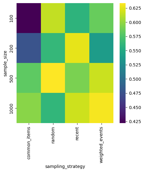
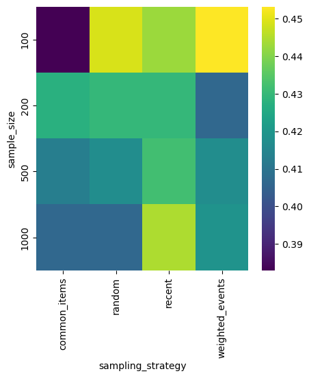
In the first experiment, we compare sampling strategies and Mean Reciprocal Rank, Precision, and Recall scores. (If you want to know more about those metrics, check the second article in the series.) Colorful plots tell better stories than tables with numbers, so let’s plot every metric as a heatmap with two dimensions: one representing sample size and the other sampling strategy.

MRR

plot_scores_heatmap(df, 'sample_size', 'sampling_strategy', 'MRR')

Precision

Recall

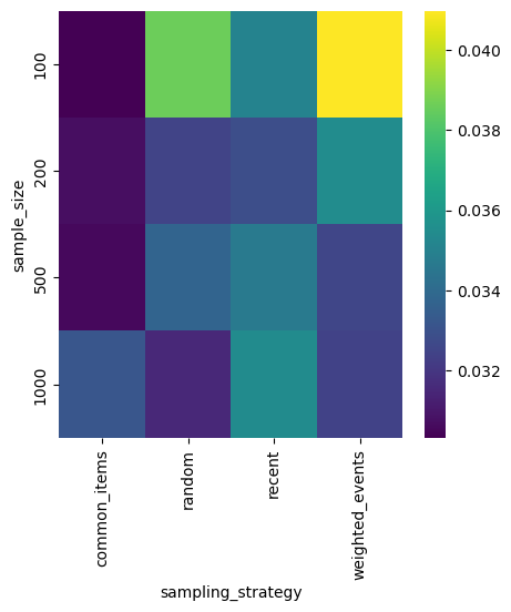
Depending on your use case, you should maximize Precision or Recall. Probably recent sampling strategy is the best, it works well for every sample size.

Experiment 2: Scoring vs Sample Size & Number of Neighbors

possible_neighbors_sizes = [250, 500, 1000, 2000]
closest_neighbors_sizes = [10, 50, 100, 250]
possible_neighbors_sampling_strategy = "recent"
number_of_recommendations = 5

experiment_2_parameters = []

for possible_n_size in possible_neighbors_sizes:
    for closest_n_size in closest_neighbors_sizes:
        experiment_2_parameters.append(
            generate_parameter_set(
                number_of_recommendations=number_of_recommendations,
                sample_size=possible_n_size,
                sampling_strategy=possible_neighbors_sampling_strategy,
                number_of_neighbors=closest_n_size
            )
        )

exp2_test = TestModels(
    training_set=training_ds,
    test_set=validation_ds,
    psets=experiment_2_parameters
)

df = exp2_test.scores()

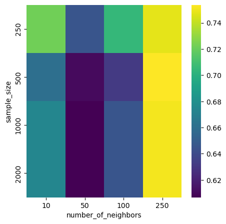
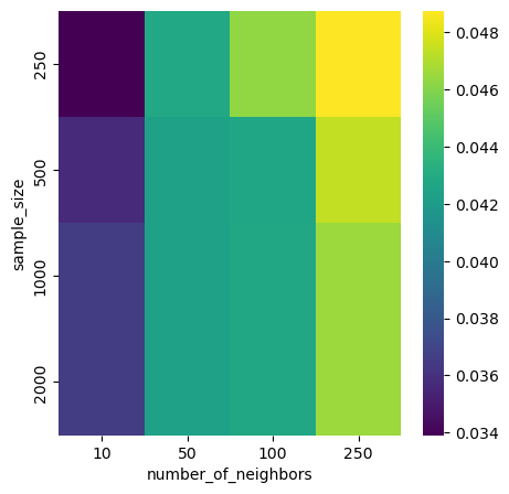
plot_scores_heatmap(df, 'sample_size', 'number_of_neighbors', 'MRR')
plot_scores_heatmap(df, 'sample_size', 'number_of_neighbors', 'Recall')
plot_scores_heatmap(df, 'sample_size', 'number_of_neighbors', 'Precision')

MRR

Recall

Precision

We clearly see that when the model picks the closest neighbors, the scoring is better.

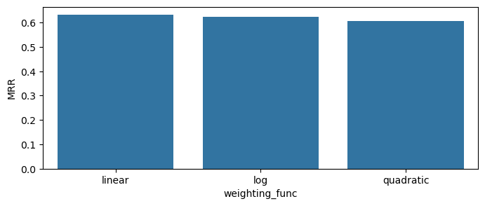
Experiment 3: Scoring vs Weighting Function

possible_neighbors_size = 1000
closest_neighbors_size = 500
neighbors_sampling_strategy = "recent"
number_of_recommendations = 5
weighting_funcs = ['linear', 'log', 'quadratic']

experiment_3_parameters = [
    generate_parameter_set(
        number_of_recommendations=number_of_recommendations,
        sample_size=possible_neighbors_size,
        sampling_strategy=neighbors_sampling_strategy,
        number_of_neighbors=closest_neighbors_size,
        weighting_func=wfunc) for wfunc in weighting_funcs
]

exp3_test = TestModels(
    training_set=training_ds,
    test_set=validation_ds,
    psets=experiment_3_parameters
)

df = exp3_test.scores()

plot_scores_barplot(df, 'weighting_func', 'MRR')
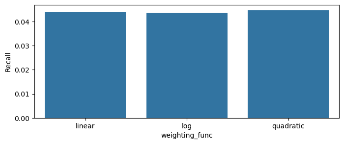
plot_scores_barplot(df, 'weighting_func', 'Recall')
plot_scores_barplot(df, 'weighting_func', 'Precision')

MRR

Recall

Precision

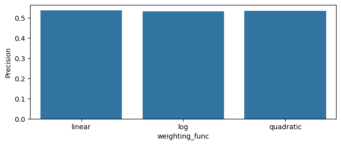
The differences between the session-weighting functions seem to be very small for this realization.

Experiment 4: Scoring vs Ranking Strategy

possible_neighbors_size = 1000
closest_neighbors_size = 500
neighbors_sampling_strategy = "recent"
number_of_recommendations = 5
weighting_func = 'log'
ranking_strategies = ['linear', 'inv', 'quadratic', 'log']

experiment_4_parameters = [
    generate_parameter_set(
        number_of_recommendations=number_of_recommendations,
        sample_size=possible_neighbors_size,
        sampling_strategy=neighbors_sampling_strategy,
        number_of_neighbors=closest_neighbors_size,
        weighting_func=weighting_func,
        ranking_strategy=r_str
    ) for r_str in ranking_strategies
]

exp4_test = TestModels(
    training_set=training_ds,
    test_set=validation_ds,
    psets=experiment_4_parameters
)

df = exp4_test.scores()

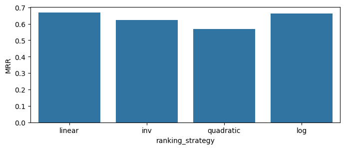
plot_scores_barplot(df, 'ranking_strategy', 'MRR')
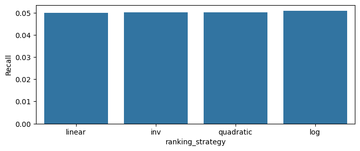
plot_scores_barplot(df, 'ranking_strategy', 'Recall')
plot_scores_barplot(df, 'ranking_strategy', 'Precision')

MRR

Recall

Precision

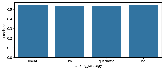
Items-weighting brings much clearer differences between weighting strategies and the model scores. We can assume that log strategy will be the best in production.

Experiment 5: Response Time vs Sample Size

The previous four experiments tested analytical scores. The model is always more than its evaluation metrics; data scientists should check other model parameters. The core engineering parameter is model response time because it might greatly limit the usefulness of the solution in a real-world setting. We will check how the model behaves when we change the size of possible neighbors’ space and sampling strategy.

sample_sizes = np.arange(1000, 10001, 200)
closest_neighbors = 250

experiment_5_parameters = []

for possible_n_size in sample_sizes:
    experiment_5_parameters.append(
        generate_parameter_set(
            sample_size=possible_n_size,
            number_of_neighbors=closest_neighbors
        )
    )

exp5_test = TestModelResponseTime(
    training_set=training_ds,
    test_set=validation_ds,
    psets=experiment_5_parameters
)

df = exp5_test.measurements()

plt.figure(figsize=(12, 6))
plt.plot(df['sample_size'], df['dt-seconds'])
plt.show()

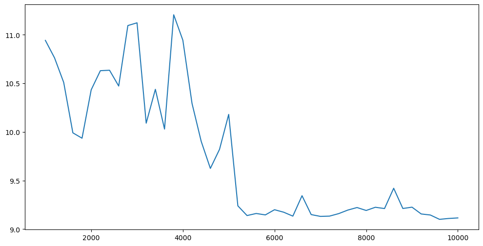
As you see, the possible neighbors’ size does not affect the response time. To be sure, you should run this experiment multiple times and check the median response time.

Experiment 6: Response Time vs Weighted & Non-weighted Items

sample_sizes = np.arange(1000, 10001, 500)
closest_neighbors = 250
methods = ['common_items', 'weighted_events', 'recent', 'random']
weight_idx = -1

experiment_6_parameters = []

for possible_n_size in sample_sizes:
    for sampling_method in methods:
        experiment_6_parameters.append(
            generate_parameter_set(
                sample_size=possible_n_size,
                number_of_neighbors=closest_neighbors,
                sampling_strategy=sampling_method,
                sampling_str_event_weights_index=weight_idx
            )
        )

exp6_test = TestModelResponseTime(
    training_set=training_ds,
    test_set=validation_ds,
    psets=experiment_6_parameters
)

df = exp6_test.measurements()

plt.figure(figsize=(12, 6))
plt.plot(df[df['sampling_strategy'] == 'common_items']['sample_size'], df[df['sampling_strategy'] == 'common_items']['dt-seconds'])
plt.plot(df[df['sampling_strategy'] == 'random']['sample_size'], df[df['sampling_strategy'] == 'random']['dt-seconds'])
plt.plot(df[df['sampling_strategy'] == 'recent']['sample_size'], df[df['sampling_strategy'] == 'recent']['dt-seconds'])
plt.plot(df[df['sampling_strategy'] == 'weighted_events']['sample_size'], df[df['sampling_strategy'] == 'weighted_events']['dt-seconds'])
plt.legend(['common_items', 'random', 'recent', 'weighted_events'])
plt.show()

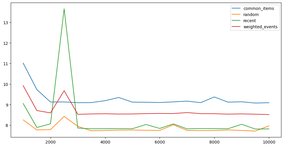
As you see, the fastest responses are generated for the random selection of possible sessions. Here, we don’t have any surprises.

Summary

Thank you for your time with the article; hopefully, you have enough knowledge to use the WSKNN system in your settings. In the next article, last from the series, we will talk more about business problems with recommendations and how to measure the business performance of our models. We will focus more on some parameters from the group because they can significantly influence the outcomes.