
Data Science: Moving Average or Moving Median for Data Filtering – Time Series
Time series are fantastic beasts that are hard to tame. Their nature may be unexpected, and we cannot use any universal method to work with them. Even filtering, the operation that should be plain and simple, plain and simple is not.
Imagine the scenario when we’re asked to build a filtering pipeline that will help us to make signals prone to anomalies. We work with the sensor placed in orbit; it measures the flow of high-energy particles from outer space. (The same scenario may be applied to different data: from the financial market or the e-commerce user behavior streams). We expect two kinds of strange behavior:
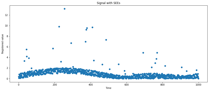
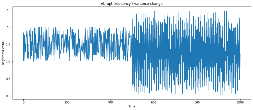
- Periods of artificial oscillations caused by our spacecraft’s abrupt change of temperature (for example, the transition from the Earth’s shadow into a full Sun illumination),
How do we build our signal filtering algorithm for those two kinds of anomalies?
Background
Time series are different than dimensionless data sources. Two main differences are:
- Values are correlated, and we can assume that the observation at time T1 will be similar to the observation at time T0. Without a weather forecasting app, we can guess that the temperature tomorrow will be within a range of today’s temperature +/- 1 degree.
- We often don’t know the future, especially in the long-range. The safe assumption is to think that time series are evolving in time and they show chaotic behavior. Just think about the stock. If we say that cryptocurrencies tend to be volatile, their price is chaotic and hard to predict.
Why do we filter data in those contexts?
The reason is to make data less noisy and easier to model. Look at Figure 1. We can distinguish there flattened sine wave. It can be modeled as a sine function if we find an appropriate frequency, phase, multiplicative factor, and additive factor. But how do we incorporate outliers in our model? The answer is: we cannot, and we shouldn’.t Outliers must be filtered out because they are not representative of our time series. The dopest thing is that if we create an optimal model that follows the usual pattern, we can detect and filter outliers quickly! We just set a threshold of difference from our forecast, and we will know about anomalies instantly, without delay.
The case in Figure 2 is more about evolution and chaotic, abrupt changes than a correlation. We see that after step 500, the frequency and amplitude of readings suddenly change, but it seems to last into the future, so we can assume that it is a “new normal.” It is not a singular event but a full-scale change of behavior. Moreover, values are changing fast, and we don’t see any outliers.
We talk about filtering, but how do we do it?
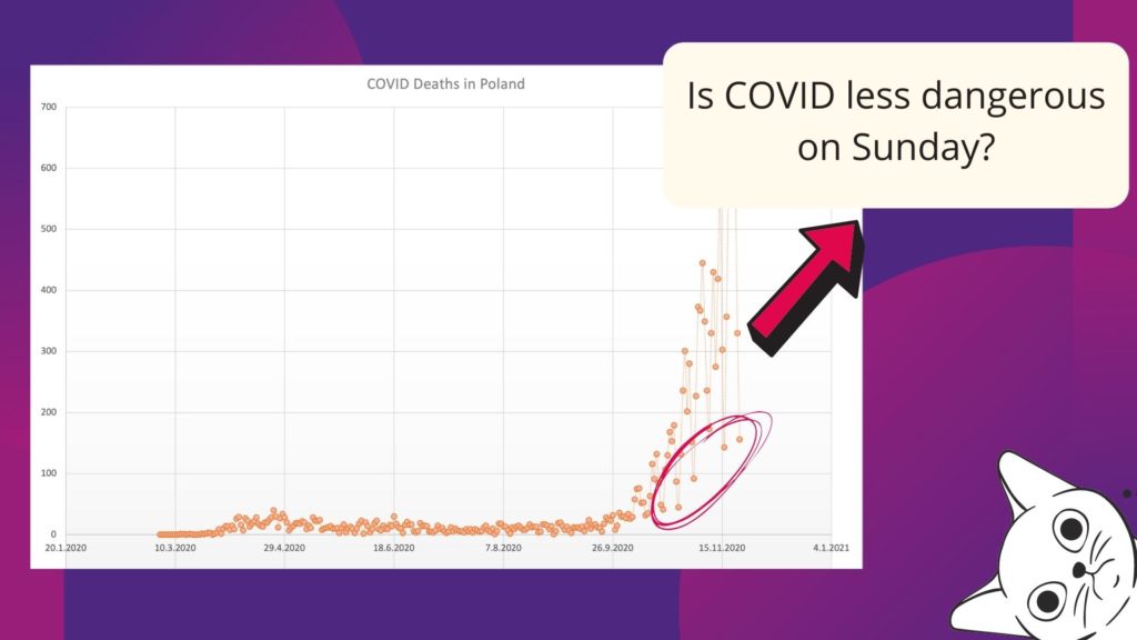
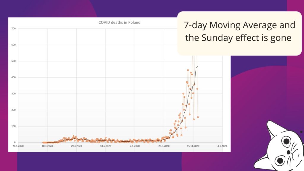
In an exploratory analysis of time-depended data, the rule of thumb is not to trust a single observation but rather to take an average (or median) of n consecutive measurements. A single value may be misleading. I don’t know how it was reported in your country, but we have seen a decreasing number of COVID deaths and cases on Sunday and a peak around Tuesday in Poland. It was related to the reporting schema and the hospital’s capacity and a data analyst should be aware of this effect. We must filter out this kind of behavior. We can group observations from a week back and use the average value to analyze the overall trend and risk associated with the disease. The same for financial data, which could be volatile, but if we aggregate it over long periods, we start to see a pattern within and without the noise.
Aggregation (filtering) leads to the loss of variance, but in return, higher-order hierarchical structures present patterns not visible at a finer scale. Decisions can be made!
Sliding Window(s) algorithms in Python
From now on, we will refer to moving windows as sliding windows. Yes, there is a different kind of moving window named expanding window, but it is not relevant for our case. Figure 5 shows the sliding window concept, and Figure 6 shows an expanding window.


How does the algorithm work?
It is straightforward: it goes through the time series from the time T + window size and aggregates values from the current time T and window size – 1 steps back. Usually, we take an average from this window as the expected value (thus, we have the Moving Average algorithm). But we can use other aggregation methods, median, standard deviation, or even exotic ones such as skewness and kurtosis.
Do you know pandas package from Python? It has many functionalities dedicated to the time series processing, and we use the method .rolling() to create a sliding-window transformer. The syntax is:
dataseries.rolling(window_size)
The .rolling() method can be applied to the pandas DataFrame and pandas Series objects with the DateTime index.
It is not the end of syntax, with only .rolling() we create an object which must be parsed with an appropriate function. It is similar to the .groupby() method. We need to pass a function over which data is aggregated/grouped. For example, if we want to calculate the moving average:
dataseries.rolling(window_size).mean()
and the moving median:
dataseries.rolling(window_size).median()
Median Filter
We can go back to our cases. The first case is a relatively stable signal with single bursts of high-energy events, and we assume that those events occur randomly. The better filter, in this case, is the median filter. Its main advantage over the classic average is its resistance to outliers. If they are rare then their amplitude doesn’t matter for the median, even if the window size is small.
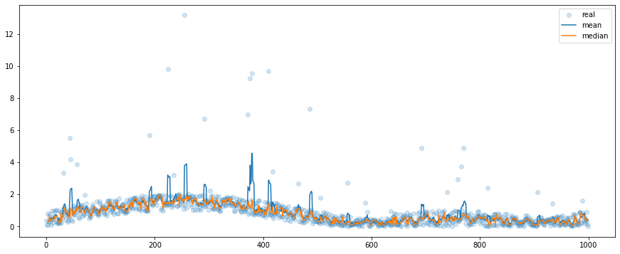
In our case, we compare the mean and median filters of window size 5 (Figure 7). We may observe that of the most time their output is similar but when it comes to outliers, the mean filter tends to follow the unexpected values. We can observe this pattern “in reality” in images with oversaturated pixels, for example from the cosmic rays. The median filter works with images and data with more dimensions too and its role is always the same: to get rid of rare artifacts.
Mean Filter
But there are cases when the median filter will fail us. Let’s take a look at how it works in comparison to the moving average from the second scenario:
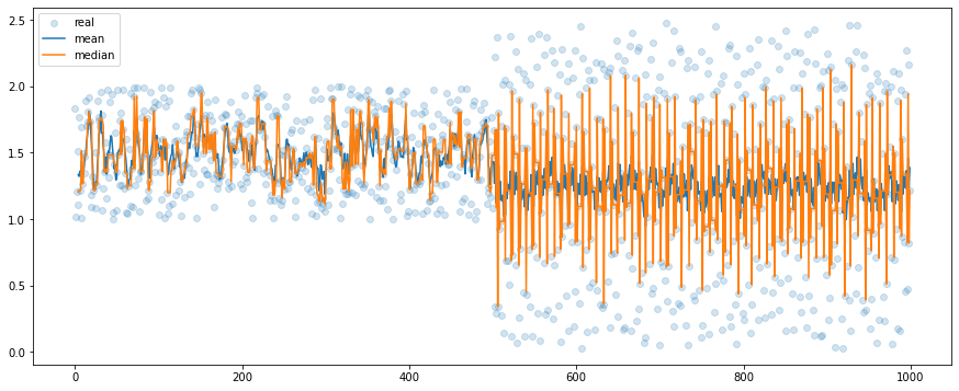
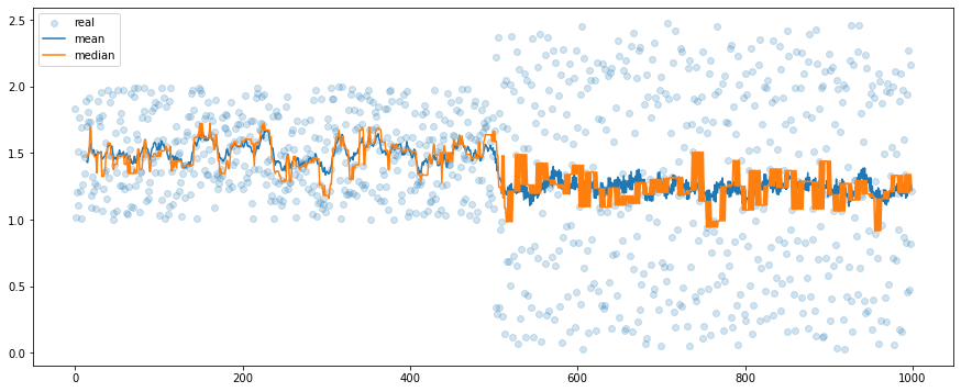
Here we don’t have outliers but high-frequency and high-amplitude signals. We have used the mean and the median filters with the window size 5. The median filter seems to be very sensitive to the volatile changes and, at the same time, the mean filter works reasonably well. Forecasts based on the median filter may quickly lose a trend in data. If this signal is responsible for the control of some device, and we use the median filter, we may damage an actuator. For data with high variance / high frequency, it is better to use the moving average. Of course, we can make the window wider, for example with a size of 15 steps, and then the mean and the median filter outputs will be similar but it is a trade-off – with larger windows, we lose more information and at some point, we may be not able to retrieve the basic properties, for example, the frequency.
Mean or Median?
We can wrap up information from this article in two sentences:
- Median filtering is better if we are removing rare events, outliers, from our dataset.
- Average filter is better for volatile and high-frequency datasets.
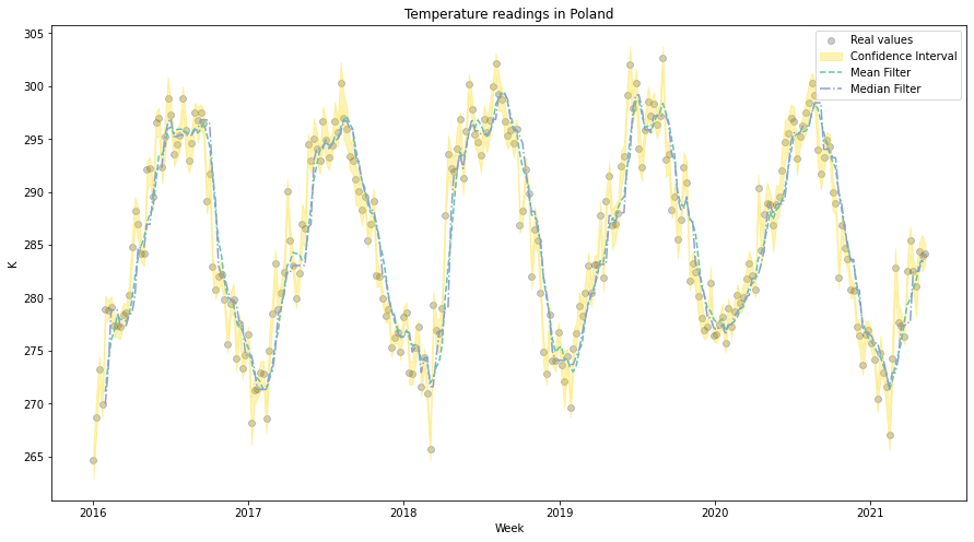
What if our data has both properties? We know that time series may evolve in an unexpected direction… Unfortunately, there are no solutions that fit all the scenarios. The best idea is to build a robust system from multiple models / filters and observe how the basic properties of our time series are changing. Sometimes, it even doesn’t matter which algorithm you use because both will work fine! We close this article with temperature readings from Poland, you may observe, that outputs from both filters are reasonably well:
Code
import numpy as np
import pandas as pd


# Alias functions

def mean_filter(dataseries: pd.Series, window_size=5):
    """
    Function applies rolling mean into given dataseries.

    Parameters
    ----------
    dataseries : pandas Series
                 Pandas Series with datetime index.

    window_size : int
                  The rolling window size, how many readings are included in a mean.

    Returns
    -------
    filtered : pandas Series
               The filtered time series.
    """

    filtered = dataseries.rolling(window_size).mean()
    return filtered


def median_filter(dataseries: pd.Series, window_size=5):
    """
    Function applies rolling mean into given dataseries.

    Parameters
    ----------
    dataseries : pandas Series
                 Pandas Series with datetime index.

    window_size : int
                  The rolling window size, how many readings are included in a mean.

    Returns
    -------
    filtered : pandas Series
               The filtered time series.
    """

    filtered = dataseries.rolling(window_size).median()
    return filtered


# Create 1st dataset

sse_data = []

for x in np.linspace(0, np.pi*2, 1000):
    t = np.random.rand()
    v = np.sin(x) + np.random.rand()
    if t > 0.95:
        v = v * np.random.randint(2, 10)
    sse_data.append(np.abs(v))

sse_data = np.array(sse_data)

# Create 2nd dataset

var_data = []

random_noise = np.random.rand(500)

var_data.extend(random_noise)

for x in np.linspace(0, np.pi*2, 500):
    t = np.random.rand()
    v = np.sin(x*220) + 0.5*t
    var_data.append(v)

var_data = (np.array(var_data)) + 1

# Filter datasets : 1

sse_avg = mean_filter(pd.Series(sse_data), 5)
sse_med = median_filter(pd.Series(sse_data), 5)

# Filter datasets : 2

var_avg = mean_filter(pd.Series(var_data), 5)
var_med = median_filter(pd.Series(var_data), 5)

# Plot the 1st

plt.figure(figsize=(15, 6))
plt.scatter(np.arange(0, 1000), sse_data, alpha=0.2)
plt.plot(sse_avg)
plt.plot(sse_med)
plt.legend(['real', 'mean', 'median'])
plt.show()

# Plot the 2nd

plt.figure(figsize=(15, 6))
plt.scatter(np.arange(0, 1000), var_data, alpha=0.2)
plt.plot(var_avg)
plt.plot(var_med)
plt.legend(['real', 'mean', 'median'])
plt.show()


[…] Moving averages help smooth out volatile data effectively. Simple moving averages treat all data points the same, while weighted moving averages focus more on recent data [3]. On top of that, median filters work better than mean-based approaches when handling outliers [4]. […]