Spatial Interpolation 101: Statistical Introduction to the Semivariance Concept

To understand Kriging we must understand semivariance first…

<< Previous part: Spatial Interpolation 101: Interpolation in Three Dimensions with Python and IDW algorithm. The Mercury Concentration in Mediterranean Sea

Don’t worry if you don’t have a geostatistical background or even if you don’t understand Kriging. I was confused when I discovered Kriging. Conceptually, the method is straightforward. But simple is not easy, and the devil is in the implementation details. The core idea behind Kriging is the semivariance concept, and we are going to uncover and understand it. The semivariance may be defined two-way: as a physical relationship between objects in space or by the statistical description of entities and their neighbors. The best-case scenario is to understand them both well. Fortunately for most of us, the concept of spatial similarity is rather obvious (but we will recall it anyway). The mathematical part is a bit more complicated, but it makes sense if we explore it with experiments.

This chapter and the following two articles uncover semivariance step by step. We start from the simple mean and standard deviation in the spatial context. In the middle part, we will analyze semivariance and covariance in one-dimensional datasets. In the last part, we are going into two dimensions with the implementation of semivariance in Excel (or Google Sheets).

Takeaways from this article

• We learn when we can use mean for spatial interpolation,
• We understand why we need to think about Confidence Intervals if we are going spatial (or temporal),
• We build a foundation for the covariance concept.
• We build a foundation for the semivariance concepet.

Physical understanding of similarity between spatial features

Let’s recall Tobler’s Law:

Everything is related to everything else, but near things are more related than distant things.

W. Tobler, 1970

What does it mean? Tobler speaks about relationships. The idea is that close things tend to be similar, and the dissimilarity increases with distance. Did you hear that long-distance relationships usually don’t work? These long-distance-related differences and short-distance-related similarities are a natural part of our physical world. We can observe those relations in multiple processes and things. So let’s skip heart issues and focus on something maybe less painful: the Land Surface Temperature readings taken by the Landsat 8 satellite.

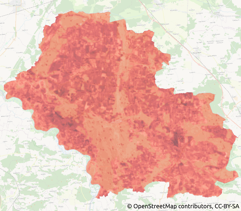
The map shows Land Surface Temperature (LST) over one county in the southern part of Poland. We can assume that if we take 10% of pixels from the LST image we will be able to reconstruct it because we know that close pixels are related to each other and they represent areas with similar temperatures! Pick a random point from the LST map and its neighbors should have similar temperatures. Take a point that is further away and the temperature will be many points above or below your first pick.

The clouds over a scene may result in missing pixels. In the previous lessons, we have exploited the Inverse Distance Weighting algorithm to retrieve missing data. We have assumed that the close points are more similar and that’s why we have used a weighting factor inversely proportional to the distance from the missing point to other points. It was Tobler Law in action. Unfortunately, there’s a problem. IDW is not the optimal solution for interpolation. Weights are fixed throughout the area but what if the weight does change with a distance? To answer this question we must take a step back and understand the semivariance, or dissimilarity concept. We start from the basic statistics and dive into more complex relations based on the mean, standard deviation and confidence interval.

Mean in action

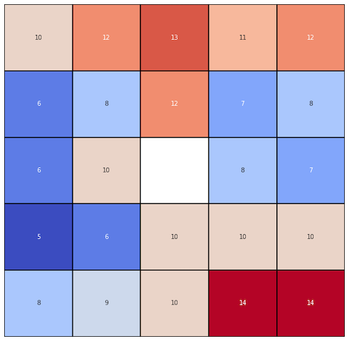
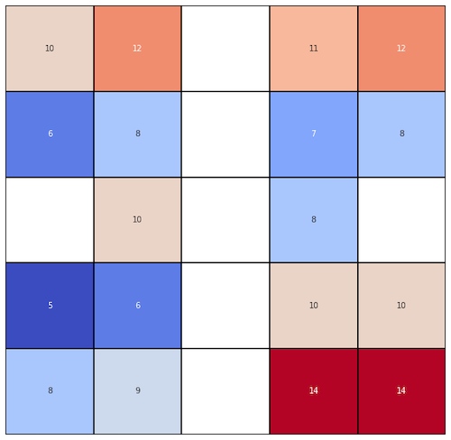
The Land Surface Temperature map is large and it’s not very useful for us because we don’t know exact pixel values. We’re going to use the small number of observations presented in the heatmap below (Figure 2).

For us, those blocks represent temperature readings at some location in the middle latitudes of the Northern Hemisphere. You may copy them into your notes if you want to perform calculations by hand. The distance between blocks is measured in units and each block is one unit apart of its neighbors in the East, West, South and North. We assume that diagonally adjacent blocks are not neighbors. You probably see interesting patterns (block grouping).

We can jump into mathematical calculations right now, but we can lose the meaning of the whole process of spatial interpolation and analysis. We won’t be so fast. We start with a statement of a simple problem.

Imagine that you have a grid of temperature sensors but one of them, in the middle of a grid, has stopped working (Figure 3). It cannot be restored right now but your job is to present the current temperature at each point. The only option is to interpolate this value. The question is:

• How to interpolate this missing value from all other values if you don’t have any specialized statistical tools?

The simple and usually right solution is to use the mean value. But mean of which concrete values? We have a few basic options:

• Mean of all values from the grid (Figure 4a),
• Mean of all values in a middle row, which represents single latitude readings (Figure 4b),
• Mean of closest neighbors (N, E, S, W) (Figure 4c),
• Mean of closest neighbors and diagonal blocks (N, NE, E, SE, S, SW, W, NW) (Figure 4d).

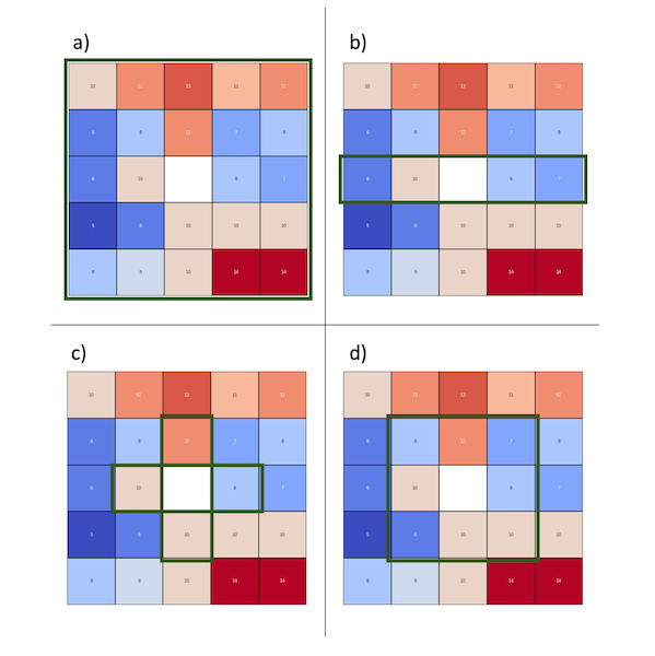
Each choice has advantages and disadvantages, so we check them all.

Missing value is a mean of all other values from the sampled grid

PROS:

• Simple solution derived from image processing where single missing pixels may be interpolated in that way.

CONS:

• Global mean may be different from the local means. We assume that distant observations are related at the same weights as close readings which is non-physical.

Missing value is a mean of values in the middle row (latitude)

PROS:

• We know from geography that temperatures at one latitude are usually similar, so this idea has a physical meaning.

CONS:

• We don’t know if latitude is the only factor which affects observed temperatures, especially if differences are small. There is a chance that the middle reading was taken on the hill and temperature may be lower; and what if this hill is a part of larger mountain range which is placed in the N-S direction?

Missing value is a mean of closest neighbors (N, S, W, E) or (N, NE, E, SE, S, SW, W, NW)

PROS:

• We assume that the closest values have the biggest influence and in a plethora of cases it is a valid assumption.

CONS:

• How many neighbors should we include in the analysis? Are all directions equally important?

Whichever method do you choose you will get slightly different results… so, which is the best? It is impossible to decide just now because there are too many loose ends. We need more information and it is hidden in the sampled data. We need to know how much neighbors affect each other, and at which distance, this connection between observations is not relevant.

For our case, where only one point is missing, the global mean of this extent is enough to produce meaningful results. We should avoid complicated methods and mental pyramids with so simple problems. The assumption that missing value is a mean of its closest neighbors is a good shot.

Moreover, even our mean is not a real mean! We can estimate set within real mean is placed, but we need for it standard deviation. This is an uncertainty, a concept that never leaves you in your geostatistical analysis.

To build confidence intervals of our prediction we should calculate Standard Deviation first. Fortunately for us, Standard Deviation is the next step from the mean into the semivariance concept!

Standard Deviation, Confidence Intervals and uncertainty of predicted mean

Standard Deviation is a measure of dispersion. Low standard deviation means that samples are close to the expected value (our mean). High Standard Deviation is a sign that our dataset covers a wide range of values and it’s not easy to find the expected value.

Throughout this tutorial we calculate the Standard Deviation of a sample, where we divide sum of variances by number of samples minus one:

$$\sigma = \sqrt{\frac{1}{N – 1} * \sum_{i=1}^N{(x_{i} – \bar{x})^2}}$$

The standard deviation of the dataset from Figure 3 is 2.58 degrees. This value tells us that variation of our dataset is not too high; we can risk the use of simple interpolation with a mean value of all samples. Then let’s do it! Divide the sum of all samples by a number of samples and you should get the value of 9.42 degrees. We will return to the concept of variation but in a slightly different form in the next lesson.

At this point, we may stop our analysis, but then we leave a very important topic of the prediction uncertainty. We can’t consider our spatial interpolation results as done without the assessment of the interpolation error. We interpolate a single value but we should think about it as a representation of some space of probable values. The estimated error tells us how wide this space is.

We can start from the uncertainty of our simple interpolation. The calculated sample mean is not exactly the process mean. Process (real) mean is somewhere within the range specified by our sample mean and confidence intervals. The real mean is somewhere between 8 and 10 degrees (Figure 5).

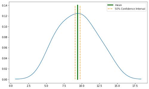
The confidence interval is not the measurement of error but it tells a lot about our interpolation! With confidence intervals, we can measure how close is our sample mean to the true mean. Yes, there is a slightly depressing fact: we can’t be 100% sure about the predicted value, it is some set of points with larger or smaller uncertainty! Anyway, in the real-world scenario, you’ll skip this problem and interpolate the missing value with the sample mean and it’s fine. We are performing a closer investigation of confidence intervals because it is an important part of statistics and if you understand it now then the more complex concepts will be easier to follow in the future.

We focus on the estimation of confidence intervals. It is a step-by-step guide on how to calculate CI from the sample. We will use values from Figure 4a.

Confidence Intervals calculation

1. Calculate degrees of freedom. We have 24 known samples; we should extract one from it (24 – 1) to calculate Degrees of Freedom. We get 23 DoF.
2. We are interested in the confidence level of 50%, or in other words, we want to be sure that there is 50% chance that our mean is within specified range.
3. Look into t-distribution table and / or calculate t statistics programmatically. I personally use scipy for such tasks, but we are doing it step by step, so we’ll look into t-distribution table. We must calculate t parameter. It is (1 – 0.5) / 2 = 0.25. Look into one tail row and find value of 0.25 then find number of DoF (column named df) which is 23 for our dataset. The cross between one tail t and DoF is our t value. You should read value t=0.685.
4. The next step is to multiply value of t (0.685) with standard deviation (2.53) divided by the square root of number of samples sqrt(24). We get value of 0.36 degree.
5. Now subtract t from mean to get the range start on the left side of our distribution and add t to the mean to get the range end on the right side of our distribution – that’s our confidence interval. There is 50% chance that our mean is located between 9.05 and 9.77 degree.

If we assume that all samples have the same weights and are independent then we can predict missing records as the mean of all other samples (9.42) with a confidence interval that the real mean of the process is between (9.42 +/- 0.36) degrees. So far it’s a nice result.

Let’s check how a situation will change if we consider scenario b) from Figure 4, where we take into account only one row of observations. As in the previous example, we will do it step by step.

1. Calculate sample mean: (6 + 10 + 8 + 7) / 4 = 7.75
2. Then degrees of freedom: 3
3. Calculate standard deviation with 3 degrees of freedom (N-1 = 3): 1.71
4. Check t-distribution table for 3 samples: 0.765
5. Calculate t value: 0.65 degree. Do you see that uncertainty is much larger with small sample size than in the case a)?
6. There is 50% chance that our real mean value is between 7.1 and 8.4 degree.

Figure 6 represents this scenario:

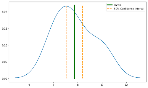
What we have learned? That smaller sample size produces larger uncertainty. With only a few samples, the space of probable results is much bigger than in Figure 5.

Is the mean value enough?

We are able to interpolate missing records at unknown locations with the mean. We can assess the uncertainty of prediction with a t-test. In a business environment, with very large datasets, it is usually the preferred technique of retrieving missing values. But it may fail you if we slightly change the whole scenario. Look into Figure 7 and think: is mean-interpolation a valid technique to retrieve multiple missing values? That’s why we need techniques as Kriging, which is built upon semivariance and covariance concepts. Which we’ll uncover in the next lesson.

Exercises:

1. Calculate mean, standard deviation and confidence intervals for scenarios c) and d). Compare results of each calculation.
2. Impute missing values from Figure 7 with global mean of available samples then calculate Root Mean Squared Error of prediction (use values from Figure 2 as the real observations). Then impute missing values with row-mean and calculate RMSE again. Which interpolation gives the better results?

Changelog

• 2021-10-03: The first release.