Spatial Interpolation 101: Interpolation in Three Dimensions with Python and IDW algorithm. The Mercury Concentration in Mediterranean Sea.

Move from the 2D interpolation into the 3D interpolation with the Inverse Distance Weighting algorithm.

<< Previous part: Spatial Interpolation 101: Interpolation of Mercury Concentrations in the Mediterranean Sea with IDW and Python

If this is your first article in the series I recommend to read the previous lesson linked above.

Transition from 2D into 3D is not so hard as it seems to be. We can easily adapt algorithm written for the 2-Dimensional IDW to perform the same operation in the n-dimensional space. In this article we are going to adapt our 2D algorithm to the new case of volumetric interpolation as well we will take a look into different styles of visualization of 3-dimensional data. Those are mostly research problems however we will tackle engineering issues too. We will write our first unit test to debug the newly created algorithm. We continue our analysis of the mercury contamination in Mediterranean Sea and we’ll build volumetric profile of the methylmercury (MeHg) concentrations.

Data Sources

• The Mercury Concentrations Dataset in this article comes from: Cinnirella, Sergio; Bruno, Delia Evelina; Pirrone, Nicola; Horvat, Milena; Živković, Igor; Evers, David; Johnson, Sarah; Sunderland, Elsie (2019): Mercury concentrations in biota in the Mediterranean Sea, a compilation of 40 years of surveys. PANGAEA, https://doi.org/10.1594/PANGAEA.899723
• And I’ve found this dataset and the article by the GEOSS search engine: Geoportal: https://www.geoportal.org
• You may check lesson’s code, notebooks, data and shapefiles here: Github repository

Environment Preparation

You should create working environment with four packages:

• numpy for the scientific computation,
• pandas for the tabular data processing and analysis,
• geopandas for the spatial data processing and analysis,
• matplotlib for the data visualization.

Install them from the conda-forge channel with Python of version from 3.6 or higher. Then download data from publication (csv file) https://doi.org/10.1594/PANGAEA.899723 along with the Mediterranean coastline shapefile from my Github (input/italy_coastline.shp).

Algorithm Development

! Code listings in this part are coming from the idw-3d-function.ipynb notebook.

Let’s imagine that you are a Data Scientist and your boss has delegated to you implementation of the algorithm which is not available in the existing Open Source packages. The question is how should you start process of implementation? We can start from the something what we shouldn’t do. We should never implement new statistical algorithms with the real-world data! Real observations are messy; and they rarely follow a easy-to-understand pattern (or distribution, if you are more into statistics). Work related to the data preparation and data cleaning may be tedious and it steals our precious time which could be devoted for the core algorithm. The right path is to create an artificial data of the well-known properties. It is easier to debug and to cover our code with tests based on the fixed dataset which is always the same, or has the same statistical properties every time when we use it. Artificial data may be created on the fly with numpy, the same package which is used for the math operations. Moreover, we are going to visualize our input data source with matplotlib package.

Our work has seven steps:

1. Generate a set of the random coordinates in a 3-dimensional space.
2. Plot the artificial points.
3. Write a function which calculates Euclidean distance between the created points and the sampled location with the unknown value.
4. Test the distance calculation function.
5. Rewrite the IDW function from the previous tutorial.
6. Test the IDW function with the prepared data.
7. Test the IDW with a generated point cloud, then interpolate unknown values and plot everything to check a result.

Step 1 – Step 2: Generate data for the algorithm development. Plot Points in the 3-Dimensional Space

How to generate the artificial data? You may do it manually but it could be a very time consuming task. The good and simple idea is to use the random numbers generator. With it we are able to create multiple 3D sets of points with random values to test and to build our algorithm. Creation of random set of coordinates in a n-dimensional space is very easy… if we utilize numpy and its random.randint() function. The arguments of this function are the lowest possible value and the highest possible value which can be picked, and the size of an output array. Function returns an array of randomly chosen integers. Listing 1 shows the random.randint() function in action. We generate an array of a random 100 coordinates in the form [x, y, z]. Then we show created points on the plane with the scatter3D() function implemented in the matplotlib package.

Listing 1: Algorithm development: random points generation and visualization

# import packages
import numpy as np
import matplotlib.pyplot as plt

# Generate 100 random arrays of 3 integer values between 0 and 1000
random_points = np.random.randint(low=0, high=1000, size=(100, 3))

# Show generated points in 3D scatterplot
figure = plt.figure(figsize=(8, 8), facecolor='w')
ax = figure.add_subplot(111, projection='3d')
ax.scatter3D(random_points[:, 0], random_points[:, 1], random_points[:, 2])
plt.show()

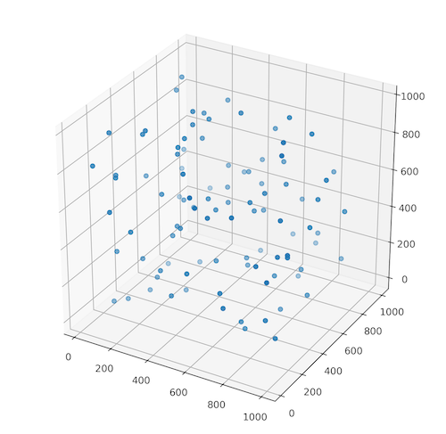
Figure 1 represents the output from the numpy.random.randint() function. Your realization is probably different because we didn’t set the random seed number which allows the reproducibility of the research. However, if you like to obtain the same points throughout the realization of the program then set the random seed to the constant value. Method for setting up the random seed in the Python program is numpy.random.seed(NUMBER).

Step 3 – Step 4: Write the function which calculates Euclidean distance between the selected set of known points and the location with unknown value. Test this function

We can calculate distance between any set of points in any dimension with the nested for loops but why should we bother with it when we can use the powerful numpy package and make calculations faster? The idea is to use the array indexing. Each column in array represents different dimension and we can quickly subtract point coordinate from each element in the column, then we can sum those and calculate square root of those sums. 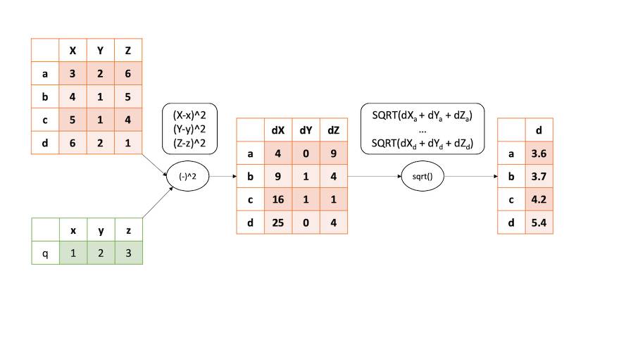Figure 2 shows this operation graphically and Listing 2 is an implementation of this process.

Listing 2: Euclidean distance calculation in n-dimensional space with numpy

def calculate_distances(coordinates, unknown_point):
    # Get coordinates dimension
    # Number of columns in numpy array / Number of dimensions
    coordinates_dim = coordinates.shape[1]  
    
    distances_between_dims = []
    
    for i in range(coordinates_dim):
        distance = (coordinates[:, i] - unknown_point[i])**2
        distances_between_dims.append(distance)
    
    dists_array = np.sqrt(np.sum(distances_between_dims, axis=0))
    
    return dists_array

Variable coordinates_dim controls the range of a for loop and by it we understand the number of dimensions of our dataset. Within the loop we are calculating distance between specific dimensions of all known points and given unknown point – we obtain list of lists with distances per dimension. Outside the loop distances are summed along each row (axis=0) and square root of those sums is a specific distance.

It is good idea to write a unit test to check if our function works as we expected. Unit test requires the hard-coded values or the special files to monitor how our script behaves. Unit tests are very useful when you develop a new package and changes in one part of it may affect functions in the other. To easily find what went wrong we run unit tests and check which one has failed. Listing 3 is the simple unit test of the output of our function. We have the hard-coded 3×3 identity matrix, the 3-element array of 2’s and the expected output which is the 3-element array of 3’s. We expect that distance from the test_arr to the test_unknown_point is always equal to 3. (You can check it manually => $\sqrt{(4 + 4 + 1)}$).

Listing 3: Unit test of the distance calculation function

# Test your algorithm with prepared array and unknown point

test_arr = np.array([
    [1, 0, 0],
    [0, 1, 0],
    [0, 0, 1]
])

test_unknown_point = [2, 2, 2]
output_distances = np.array([3, 3, 3])

distances = calculate_distances(coordinates=test_arr, unknown_point=test_unknown_point)

assert (distances == output_distances).all()  # Here is a test

Hopefully our function has passed the test and we are able to move to the next step of an algorithm development.

Step 5: Rewrite IDW function from previous tutorial

In the previous lesson our IDW function was designed only for the two-dimensional data. Let’s recall it (Listing 4).

Listing 4: The two-dimensional IDW function

def inverse_distance_weighting(unknown_point, points, power, ndist=10):

    distances = calculate_distances(points, unknown_point)
    points_and_dists = np.c_[points, distances]
    
    # Sort and get only 10 values
    points_and_dists = points_and_dists[points_and_dists[:, -1].argsort()]
    vals_for_idw = points_and_dists[:ndist, :]
    
    # Check if first distance is 0
    if vals_for_idw[0, -1] == 0:
        return vals_for_idw[0, 2]
    else:
        # If its not perform calculations
        weights = 1 / (vals_for_idw[:, -1]**power)
        numerator = weights * vals_for_idw[:, 2]
        interpolated_value = np.sum(numerator) / np.sum(weights)
        return interpolated_value

What must be changed to use this function for the any number of dimensions?

We assume that the function argument points is an array of coordinates and their respective measurements. As example: [LAT, LON, DEPTH, MERCURY CONCENTRATION]. We cannot pass all the values for the distance calculation, thus we use numpy’s indexing to pass only the geographical coordinates and a depth. Instead of:

distances = calculate_distances(points, unknown_point)

We are going to write:

distances = calculate_distances(points[:, :-1], unknown_point)

And instead of:

points_and_dists = np.c_[points, distances]

We change it to:

vals_and_dists = np.c_[points[:, -1], distances]

In the first change we pass only the coordinates to the calculate_distances() function. The second change is analogical to the first one but this time we pass all rows and only the last column to the new array of the observed values and distances between them and the point of unknown value.

Finally we get an array with two elements: [known point value, distance between known point and unknown point]. As you may noticed we’ve changed variable name from points_and_dists to vals_and_dists. It is a naming convention derived from the clean code: the variable name should be descriptive and it definitively shouldn’t be misleading.

The sorting part doesn’t change. We must check if the first value in a sorted list is different than 0. From this point the main difference is related to the array indexing which you may see in the code Listing 5 with a full implementation of this function. The main problem is a distance calculation function. If we build it to work with the n-dimensional data then our IDW function will work without any problems.

Listing 5: Multidimensional IDW function

def inverse_distance_weighting(unknown_point, points, power, ndist=10):
    """
    Function estimates values in unknown points with with inverse weighted interpolation technique.
    
    INPUT:
    :param unknown_point: coordinates of unknown point,
    :param points: (array) list of points and they values [dim 1, ..., dim n, val],
    :param power: (float) constant used to calculate IDW weight -> weight = 1/(distance**power),
    :param ndist: (int) how many closest distances are included in weighting,
    
    OUTPUT:
    :return interpolated_value: (float) interpolated value by IDW method.
    
    Inverse distance weighted interpolation is:
    
    est = SUM(WEIGHTS * KNOWN VALS) / SUM(WEIGHTS)
    and
    WEIGHTS = 1 / (DISTANCE TO UNKNOWN**power)
    
    where:
    power is a constant hyperparameter which tells how much point is influenced by other points. 
    """

    distances = calculate_distances(points[:, :-1], unknown_point)
    vals_and_dists = np.c_[points[:, -1], distances]
    
    # Sort and get only 10 values
    vals_and_dists = vals_and_dists[vals_and_dists[:, 1].argsort()]
    vals_for_idw = vals_and_dists[:ndist, :]
    
    # Check if first distance is 0
    if vals_for_idw[0, 1] == 0:
        # If first distance is 0 then return first value
        return vals_for_idw[0, 0]
    else:
        # If it's not perform calculations
        weights = 1 / (vals_for_idw[:, 1]**power)
        numerator = weights * vals_for_idw[:, 0]
        interpolated_value = np.sum(numerator) / np.sum(weights)
        return interpolated_value

Step 6: Test IDW function

As we’ve tested the distance calculation, we are going to test IDW algorithm too. The idea is the same, we create the hard-coded arrays and check if the output is the same as it should be based on the manual calculations. Listing 6 is the test for it.

Listing 6: Unit test of Inverse Distance Weighting function

test_arr = np.array([
    [1, 0, 0, 1],
    [0, 1, 0, 1],
    [0, 0, 1, 1]
])

test_unknown_point = [2, 2, 2]

output_est = 1

estimated_value = inverse_distance_weighting(test_unknown_point, test_arr, 2)

assert output_est == estimated_value

Step 7: Test IDW with artificial data

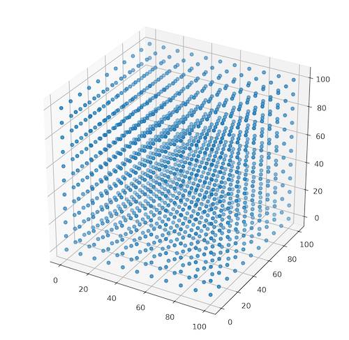
To close the part with a function development we will test it with the randomly generated points. We should create a evenly spaced set of points in the 3-dimensional space (Figure 3). We can achieve it within numpy with two operations: the coordinates generation and their positioning (Listing 7).

Listing 7: Function for creation of evenly spaced points cloud

def generate_coordinates(lower, upper, step_size, dimension):
    coordinates = [np.arange(lower, upper, step_size) for i in range(0, dimension)]
    mesh = np.hstack(np.meshgrid(*coordinates)).swapaxes(0, 1).reshape(dimension, -1).T
    return mesh
coords = generate_coordinates(0, 101, 10, 3)

The method from the Listing 7 uses numpy.arange() function to generate an array with coordinates from the lower to the upper limit and then it uses numpy.meshgrid() to create all possible realizations (permutations) of the points in a space of size controlled by a given dimension (Figure 3). Unfortunately for us, all of those points are only coordinates without any value. We must generate sample of random points in the same space, but this time with assigned values. This could be done with function from Listing 1. Only difference is the number of records in a row, then it was three (x, y, z) and now we need four (x, y, z, value). One realization of this function is presented in the Listing 8 and Figure 4 shows the generated set of points.

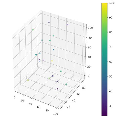
Listing 8: Random sample of values in 3D space.

# Generate points with values

known_points = np.random.randint(0, 101, size=(20, 4))

# Show known points

figure = plt.figure(figsize=(8, 8), facecolor='w')
ax = figure.add_subplot(111, projection='3d')
p = ax.scatter3D(known_points[:, 0], known_points[:, 1], known_points[:, 2],
             c=known_points[:, -1], cmap='viridis')
figure.colorbar(p)
plt.show()

The result of our work up to this moment is a 3D canvas of evenly spaced points and few samples for interpolation. We are able to perform interpolation and to fill the canvas with values. We will store output as the new numpy array of rows with [x, y, z, interpolated value] and to do so, we are going to iterate through each record of the empty canvas. Listing 10 shows function which performs this process and Figure 5 presents the resulting grid.

Listing 9: Interpolate values from canvas.

def interpolate_values(array_of_coordinates, array_of_known_points):
    output_arr = []
    
    for row in array_of_coordinates:
        interpolated = inverse_distance_weighting(row, array_of_known_points, power=3, ndist=5)
        interpol_arr = np.zeros(shape=(1, len(row) + 1))
        interpol_arr[:, :-1] = row
        interpol_arr[:, -1] = interpolated
        output_arr.append(interpol_arr[0])
        
    return np.array(output_arr)

interp = interpolate_values(coords, known_points)

# Show interpolation results

figure = plt.figure(figsize=(12, 12), facecolor='w')
ax = figure.add_subplot(111, projection='3d')
p = ax.scatter3D(interp[:, 0], interp[:, 1], interp[:, 2],
             c=interp[:, -1], cmap='viridis')
figure.colorbar(p)
plt.show()

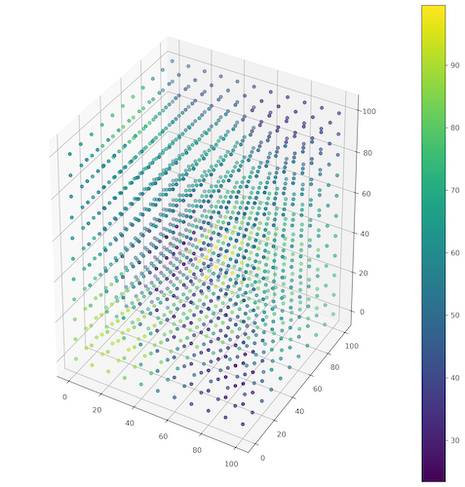
Congratulations! We’ve created the IDW algorithm for interpolation of the points values in the 3D space! Finally, we are going to work with the real world data!

Data Preparation

! Code listings in this part are coming from the idw-3d-and-mercury-concentrations-data-prep.ipynb notebook.

We are using similar procedure of a data preparation as in the previous tutorial. The significant difference is that we are going to use all dates of measurements and we limit the extent to the coastline of Italy. Download data from here and open new Jupyter Notebook. Import pandas and read csv file with observations with pandas.read_csv() method. Create a copy of a DataFrame with columns [‘lon’, ‘lat’, ‘depth_m’, ‘mea_ug_kg_orig’] which are: longitude, latitude, depth, mean concentration of Hg in the sampled organisms (Listing 10).

Listing 10: Read and prepare DataFrame with observations

import pandas as pd

# Read dataframe

df = pd.read_csv('input/190516_m2b_marine_biota.csv', sep=';', encoding = "ISO-8859-1", index_col='id')

# Get only columns: ['lon', 'lat', 'depth_m', 'mea_ug_kg_orig']

cols = ['lon', 'lat', 'depth_m', 'mea_ug_kg_orig']

ndf = df[cols]

As we decided earlier we limit the study extent to the Italian coast and to the maximum sampling depth of 20 meters. Study extent is defined by the extremities: 35.3N – 47.05N; 6.37E – 18.31E. With numpy array indexing we are able to limit area of the study to the specific area within a given coordinates (Listing 11).

Listing 11: Defining study extent with pandas DataFrame indexing

# Limit data by latitude and longitude and depth
# Latitude limits: 35.3N - 47.05N
# Longitude limits: 6.37E - 18.31E
# Depth limit: 0m - 20m

lat_limit_bottom = ndf['lat'] > 35.3
lat_limit_top =  ndf['lat'] < 47.05

lon_limit_bottom = ndf['lon'] > 6.37
lon_limit_top =  ndf['lon'] < 18.31

depth_limit_top = ndf['depth_m'] >= 0  # inverted!
depth_limit_bottom = ndf['depth_m'] < 20

ndf = ndf[lat_limit_bottom & lat_limit_top & lon_limit_bottom & lon_limit_top
         & depth_limit_bottom & depth_limit_top]

Created DataFrame has 2387 records and we assume that it is enough for the analysis. We should store transformed data and it can be done with the method pandas.to_csv(). In this tutorial we’ll name output file as the prepared_data_mercury_concentrations_volumetric.csv. You can download this file from the tutorial repository if you’ve skipped the step of a data prepration.

Analysis

! Code listings in this part are coming from the idw-3d-analysis.ipynb notebook.

At the beginning of this lesson we’ve developed tools for data analysis. Then we’ve prepared dataset. Now it’s time for something far more interesting. Finally we are going to join our materials (data) and tools (algorithms) to perform spatial analysis. Our work here is straightforward with one exception at the end of the project. This part of the project requires import of a standard Spatial Data Science libraries (pandas, geopandas, numpy) and matplotlib.pyplot for the visualization. We’ll import ScalarMappable class from matplotlib.cm and use it in the last part of the exercise for the colorbar plotting.

Start with loading of:

• prepared_data_mercury_concentrations_volumetric.csv file with pandas,
• italy_coastline.shp with geopandas (Listing 12).

Listing 12: Import packages and load data for analysis

import pandas as pd
import geopandas as gpd
import numpy as np

import matplotlib.pyplot as plt
from matplotlib.cm import ScalarMappable

# 1. Read data.

df = pd.read_csv('prepared_data_mercury_concentrations_volumetric.csv', sep=',', encoding='utf8', index_col='id')
gdf = gpd.read_file('input/italy_coastline.shp')
gdf.set_index('id', inplace=True)

The good idea is to check our DataFrame before we start an analysis. The mercury concentrations table should look like:

id	lon	lat	depth_m	mea_ug_kg_orig
1169	12.5	44.9	5.0	114.0
9577	14.0	43.8	10.0	22.0

With geopandas we are able to plot our GeoDataFrame and check visually if everything is ok with the geometry. Use for it gdf.plot() method. We may inspect geometry type too, just need to print geometry attribute of the GeoDataFrame with gdf.geometry command. In our case it is the MultiPoint type.

The hardest part: build the volumetric profile of the coastline and perform inverse distance weighting. For the sake of simplicity, we skip the real depths and we build five depth levels for each point (0, 5, 10, 15, 20 meters). We can create the new DataFrame with columns for each level, but there is an option to create those profiles when interpolation algorithms runs, so we will use this opportunity. Now it is hard to imagine how will we do it, but Figure 6 shows algorithm to make it clearer. We have to write four functions to achieve the final result. Three of them already exist and those are: calculate_distances() from Listing 2, inverse_distance_weighting() from Listing 5 and interpolate_values() from Listing 9 which will be slightly changed for the needs of our process.

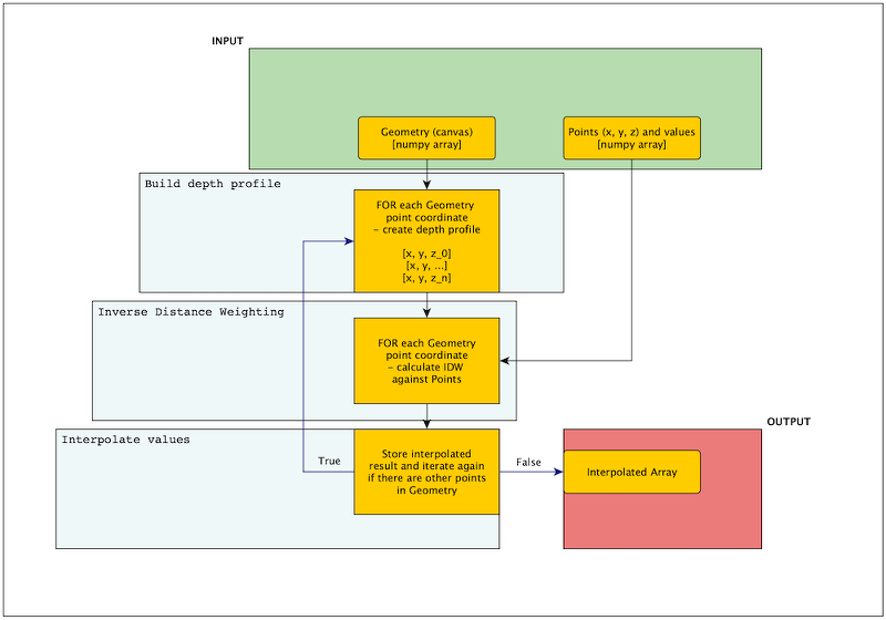
Algorithm for 3D IDW is complicated but complexity comes from the depth profile building. Without this step, as example if we provide the pre-defined canvas, then process is straightforward. Look into list below, the italic paragraphs are the algorithm without the depth profile building and the bold paragraph describes place of the additional step of the depth profile creation:

• iterate through each point where you want to interpolate values (here it is the Geometry object from the Figure 6),
• build depth profiles for the specific unknown point and return array with a series with points and the specific depths, as example: [ [x, y, 0], [x, y, 5], [x, y, 10] ] where we have three depth levels,
• perform inverse distance weighting on those points with the array containing points of the known values (here it is the Points object from the Figure 6),
• assign a interpolated value to the point and return it.

All values should be passed into the interpolate_values() function (Listing 13 is a changed function). Then, in the loop, each unknown point from canvas is transferred to the build_depth_profile() function (Listing 14). From there the array with depth profiles is returned again to interpolate_values() and for each depth of this array inverse distance weighting is applied to the canvas points. Then the interpolated value is stored in the array. When all points are interpolated then output array is returned, and we can visualize it.

Listing 13: Interpolate values, updated function

def interpolate_values(array_of_coordinates, array_of_known_points):
    output_arr = []
    
    for row in array_of_coordinates:
        pts = build_volumetric_profile_array(row[0]) # Here is an update
        for pt in pts:
            interpolated = inverse_distance_weighting(pt, array_of_known_points, power=3, ndist=5)
            interpol_arr = np.zeros(shape=(1, len(pt) + 1))
            interpol_arr[:, :-1] = pt
            interpol_arr[:, -1] = interpolated
            output_arr.append(interpol_arr[0])
        
    return np.array(output_arr)

Listing 14: Build depth profile

def build_volumetric_profile_array(points):
    """Function adds depth levels to the coastline geometry"""
    ranges = np.arange(0, 21, 5)
    mpts = []
    for r in ranges:
        vals = [points[0].x, points[0].y, r]
        mpts.append(vals)
    return np.array(mpts)

Now we move to the very interesting part of the data visualization in multiple dimensions. We have done it before (Listing 9) and we will do it again. Here’s a bit of advice: our depth profiles are positive integers so our visualization will be inverted (deepest part will be at the top). To change this behavior you can modify function from Listing 14 to produce negative values, or you can invert axis in matplotlib. To do the latter we use ax.invert_zaxis() method (Figure 7).

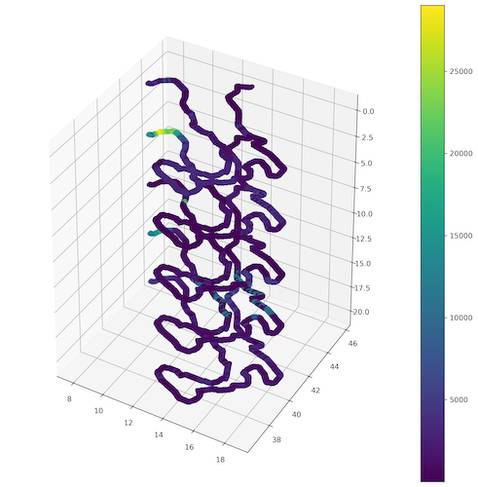
Ok… there are some patterns but unfortunately plot is not readable! It is hard to distinguish specific points and values!

Three or more dimensional data visualization is tricky. The good idea is to change plot to the series of 2-dimensional scatter plots to show how values are changed within the depth. This is not so easy task and I was struck with it when I wanted to plot colorbar. Fortunately, there is a method to do it. We’ve mentioned earlier that we must import ScallarMappable class from matplotlib. Here’s the use of it. We are going to build a colorbar based on the assumptions that the minimum concentration of MgHg is 0 and maximum is 30 000. Whole process is presented in the Listing 15.

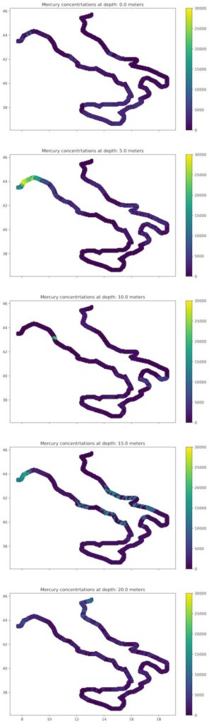
Listing 15: Plot multiple depth profiles as a series of plots

# Get unique depths

unique_depths = np.unique(interpolated[:, 2])

# Prepare figures

scale = np.linspace(0, 30000, 300)
cmap = plt.get_cmap('viridis')
norm = plt.Normalize(scale.min(), scale.max())
sm = ScalarMappable(norm=norm, cmap=cmap)
sm.set_array([])

fig, axes = plt.subplots(nrows=5, ncols=1, sharex=True, figsize=(10, 35))

for idx, depth_level in enumerate(unique_depths):
    
    x = interpolated[:, 0][interpolated[:, 2] == depth_level]
    y = interpolated[:, 1][interpolated[:, 2] == depth_level]
    col = interpolated[:, -1][interpolated[:, 2] == depth_level]
    
    axes[idx].scatter(x, y, c=col, vmin=0, vmax=30000, cmap='viridis')
    axes[idx].set_title('Mercury concentrtations at depth: {} meters'.format(depth_level))
    
    fig.colorbar(sm, ax=axes[idx])

Figure 8 is better for comparison between the depths. This teaches us that it is better to distribute data among multiple plots if it will be analyzed by the human-expert. The same approach may be used for the time-series presentation or other 3-dimensional datasets.

Ok, that’s all. We have created full algorithm for the3D IDW and now we are able to perform IDW in a n-dimensional space. Additionally, we know how to plot a 3D data to preserve meaningful information and reduce noise related to the overlapping points. Listing 16 is a full algorithm to perform this kind of analysis. Feel free to use it and share it!

Listing 16: Full code for 3D IDW interpolation

import pandas as pd
import geopandas as gpd
import numpy as np

import matplotlib.pyplot as plt
from matplotlib.cm import ScalarMappable

# 1. Read data.
# 2. Check data.
# 3. Prepare model(geometry).
# 4. Interpolate missing values.
# 5. Visualize output.

# 1. Read data.

df = pd.read_csv('prepared_data_mercury_concentrations_volumetric.csv', sep=',', encoding='utf8', index_col='id')
gdf = gpd.read_file('input/italy_coastline.shp')
gdf.set_index('id', inplace=True)

# 3. Prepare model(geometry).

# For each point add depth profile - create new dataframe with those points

def build_volumetric_profile_array(points):
    """Function adds depth levels to the coastline geometry"""
    ranges = np.arange(0, 21, 5)
    mpts = []
    for r in ranges:
        vals = [points[0].x, points[0].y, r]
        mpts.append(vals)
    return np.array(mpts)

# 4. Interpolate missing values.
# 4. Calculate distances between 3D coordinates list and unknown point. Use numpy array operations.

def calculate_distances(coordinates, unknown_point):
    # Get coordinates dimension
    coordinates_dim = coordinates.shape[1]  # Number of columns in numpy array / Number of dimensions
    
    distances_between_dims = []
    
    for i in range(coordinates_dim):
        distance = (coordinates[:, i] - unknown_point[i])**2
        distances_between_dims.append(distance)
    
    dists_array = np.sqrt(np.sum(distances_between_dims, axis=0))
    
    return dists_array

def inverse_distance_weighting(unknown_point, points, power, ndist=10):
    """
    Function estimates values in unknown points with with inverse weighted interpolation technique.
    
    INPUT:
    :param unknown_point: coordinates of unknown point,
    :param points: (array) list of points and they values [dim 1, ..., dim n, val],
    :param power: (float) constant used to calculate IDW weight -> weight = 1/(distance**power),
    :param ndist: (int) how many closest distances are included in weighting,
    
    OUTPUT:
    :return interpolated_value: (float) interpolated value by IDW method.
    
    Inverse distance weighted interpolation is:
    
    est = SUM(WEIGHTS * KNOWN VALS) / SUM(WEIGHTS)
    and
    WEIGHTS = 1 / (DISTANCE TO UNKNOWN**power)
    
    where:
    power is a constant hyperparameter which tells how much point is influenced by other points. 
    """

    distances = calculate_distances(points[:, :-1], unknown_point)
    vals_and_dists = np.c_[points[:, -1], distances]
    
    # Sort and get only 10 values
    vals_and_dists = vals_and_dists[vals_and_dists[:, 1].argsort()]
    vals_for_idw = vals_and_dists[:ndist, :]
    
    # Check if first distance is 0
    if vals_for_idw[0, 1] == 0:
        # If first distance is 0 then return first value
        return vals_for_idw[0, 0]
    else:
        # If it's not perform calculations
        weights = 1 / (vals_for_idw[:, 1]**power)
        numerator = weights * vals_for_idw[:, 0]
        interpolated_value = np.sum(numerator) / np.sum(weights)
        return interpolated_value

def interpolate_values(array_of_coordinates, array_of_known_points):
    output_arr = []
    
    for row in array_of_coordinates:
        pts = build_volumetric_profile_array(row[0])
        for pt in pts:
            interpolated = inverse_distance_weighting(pt, array_of_known_points, power=3, ndist=5)
            interpol_arr = np.zeros(shape=(1, len(pt) + 1))
            interpol_arr[:, :-1] = pt
            interpol_arr[:, -1] = interpolated
            output_arr.append(interpol_arr[0])
        
    return np.array(output_arr)

geometry_array = gdf.to_numpy()
interpolated = interpolate_values(geometry_array, df.to_numpy())

# 5. Visualize output.

# Get unique depths

unique_depths = np.unique(interpolated[:, 2])

# Prepare figures

scale = np.linspace(0, 30000, 300)
cmap = plt.get_cmap('viridis')
norm = plt.Normalize(scale.min(), scale.max())
sm = ScalarMappable(norm=norm, cmap=cmap)
sm.set_array([])

fig, axes = plt.subplots(nrows=5, ncols=1, sharex=True, figsize=(10, 35))

for idx, depth_level in enumerate(unique_depths):
    
    x = interpolated[:, 0][interpolated[:, 2] == depth_level]
    y = interpolated[:, 1][interpolated[:, 2] == depth_level]
    col = interpolated[:, -1][interpolated[:, 2] == depth_level]
    
    axes[idx].scatter(x, y, c=col, vmin=0, vmax=30000, cmap='viridis')
    axes[idx].set_title('Mercury concentrtations at depth: {} meters'.format(depth_level))
    
    fig.colorbar(sm, ax=axes[idx])

Exercises:

1. Refactor the code and create a class for the IDW calculation. This class should have all functions (methods) from the lesson. Think about the class arguments (parameters) which should be included during the object initialization.
2. Think how to visualize a 4-dimensional dataset. As example [lon, lat, depth, time]? Is there a good way to do it? What are the trade-offs of each way?
3. There is one particular problem related to our analysis: we assume that the depth has the same spatial dimension as the lon/lat coordinates and this is not true. How to enhance algorithm to support different scales? (We will answer this question in the future, but feel free to experiment with this issue).

Next Lesson

Sample mean, standard deviation and confidence intervals. The foundation for the semivariance concept.

Bibliography

[1] Health Effects of Exposures to Mercury. United States Environmental Protection Agency. Link: https://www.epa.gov/mercury/health-effects-exposures-mercury

[2] EPA-FDA Fish Advice: Technical Information. United States Environmental Protection Agency. Link: https://www.epa.gov/fish-tech/epa-fda-fish-advice-technical-information

[3] Github with article’s notebooks and shapefiles

[4] Cinnirella, Sergio; Bruno, Delia Evelina; Pirrone, Nicola; Horvat, Milena; Živković, Igor; Evers, David; Johnson, Sarah; Sunderland, Elsie (2019): Mercury concentrations in biota in the Mediterranean Sea, a compilation of 40 years of surveys. PANGAEA, https://doi.org/10.1594/PANGAEA.899723

Changelog

• 2021-07-18: The first release.