Spatial Interpolation 101: Interpolation of Mercury Concentrations in the Mediterranean Sea with IDW and Python

Build your first spatial interpolation algorithm in Python

<< Previous part: Spatial Interpolation 101: Introduction to Inverse Distance Weighting Interpolation Technique

Spatial interpolation techniques are very useful tools for environmental protection cases. Imagine that we have to perform analysis of the soil composition near open pit mine. It could be very expensive to sample each square meter of this area. We’re not able to take thousands of samples, but few dozens is within our reach. With those hundred available we can perform interpolation to estimate area’s contamination levels at unsampled locations.

We can use multiple interpolation techniques for this task. Inverse Distance Weighting (IDW) is one of them and we are going to uncover it in this lesson. It is the simplest and good for building vanilla model for further tuning.

In this article we’ll use IDW for interpolation of mercury concentrations near the coast of the Mediterranean Sea.

We’ll learn how to:

• Implement Inverse Distance Weighting algorithm in Python and Numpy,
• Transform spatial data for modeling purposes.

Data Sources

• Mercury concentrations dataset in this article comes from: Cinnirella, Sergio; Bruno, Delia Evelina; Pirrone, Nicola; Horvat, Milena; Živković, Igor; Evers, David; Johnson, Sarah; Sunderland, Elsie (2019): Mercury concentrations in biota in the Mediterranean Sea, a compilation of 40 years of surveys. PANGAEA, https://doi.org/10.1594/PANGAEA.899723
• And I’ve found this dataset and article by the GEOSS search engine: Geoportal: https://www.geoportal.org
• You may check lesson’s code, notebooks, data and shapefiles here: Github repository

Theoretical Background

Mercury is a neurotoxin. It accumulates in sea organisms and indirectly in our bodies as a methylmercury (MeHg). U.S. EPA guidelines tells us that methylmercury in high concentrations:

• affects our sight (loss of peripheral vision),
• affects our muscles (weakness of muscle, impaired coordination, problems with speech, hearing and walking),
• changes our neural responses and creates anxious sensation of “pins and needles”, usually in the hands, feet, and around the mouth,
• is very dangerous for unborn infants’ brains and nervous systems [1].

There are some publications that MeHg may cause tumors, but there are others which show no significant effects of exposure to MeHg and cancer development. We should be cautious with conclusions on this topic; however, the risk of the central nervous system damage in adults and extremely high threat for the fetus’ brain and neural development is enough to monitor mercury concentration in sea organisms which, for some world populations, are the main food source.

Data modeling pipeline and programming environment preparation

Data modeling pipeline for each data science problem is very similar. Steps from programming environment preparation up to the model development are as follows:

1. (Environment Preparation) Anaconda setup.
2. (Environment Preparation) Installation of Python Packages.
3. (Data) Data download.
4. (Data) Data processing and transformation.
5. (Data) Data exploration.
6. (Model) Model Development.
7. (Model) Model Implementation.

In this tutorial we cover points 4-6. I expect that you can set up Anaconda and it’s environment and install necessary Python packages. (If I’m wrong please tell me in a comment section, then I’ll prepare short article how to set up environment and install Anaconda in MacOS and/or Linux systems).

Our programming environment has five Python packages:

• numpy for scientific computation,
• pandas for tabular data processing and analysis,
• geopandas for spatial data processing and analysis,
• matplotlib for data visualization,
• seaborn for data visualization.

Install them from the conda-forge channel with Python of version from 3.6 or above. Then download data from publication (csv file) https://doi.org/10.1594/PANGAEA.899723 along with Mediterranean coastline shapefile from my Github (medi_coastline.shp).

We are ready to go!

Data preparation and exploration

Code listings from this part are included in the idw-data-exploration.ipynb notebook.

Before we start modeling it is a good idea to look into a dataset. We read csv file with Pandas, slice dataset and store it as a new csv file for model development. We don’t need all information provided by authors for our purposes. Listing 1 shows how to read data and look into it.

Listing 1: Data exploration: read csv file

import pandas as pd

df = pd.read_csv('190516_m2b_marine_biota.csv',
                 sep=';', encoding = "ISO-8859-1",
                 index_col='id')

print(df.head())

Our DataFrame has 36 columns. What columns are avaliable? And how many rows has our dataset? Let’s check it (Listing 2).

Listing 2: Data exploration: check columns and number of records in a dataset

print('Columns in dataframe:')
for idx, col in enumerate(df.columns):
    print(idx+1, col)

print('Dataframe length:', len(df))

From those columns we are interested in:

• lat (latitude),
• lon (longitude),
• mea_ug_kg_orig (mean Hg concentrations in a sampled organisms).

But still, we have more than 24 thousand rows of data… It is a good idea to take only a part of DataFrame for a model development. We rather not use entire data set when we are building model from scratch. Why? Two main reasons are:

1. New code is (usually) not optimized from the computational perspective and if you test its output and logic you need to do it as fast as possible,
2. Sometimes data is flawed in some way and it is hard to find which records are corrupted. It is easier to find those corrupted records in small dataset than a big one.

How do we divide our dataset? We can do it by the date of sampling and limit records to those sampled in the 21^st century. The icing on the cake here is that measurements taken in the less distant past from today should be considered as closer to the current state of Hg concentrations and more important from the policy-making perspective. Listing 3 shows process of data division by time with Pandas time-indexing. In the first step we create new column with sampling dates formatted as datetime pandas object. Next we check how many records are available after 2000s and in the last step we create the new DataFrame with limited number of records (Listing 3).

Listing 3: Data exploration: sampling records by the date of observation

df['samp_date'] = pd.to_datetime(df['samp_date'],
                                 format='%Y-%M-%d')
updated_df = df[df['samp_date'] > '2000-01-01']

print(len(df['samp_date'][df['samp_date'] > '2000-01-01']))

Before we export updated_df to the csv file we are going to slice it, and we’ll leave only lat, lon and mea_ug_kg_orig columns. Then we save our final DataFrame (Listing 4).

Listing 4: Data exploration: save prepared DataFrame to csv

ndf = updated_df[['lat', 'lon', 'mea_ug_kg_orig']]
ndf.to_csv('prepared_data_mercury_concentrations.csv',
            encoding='utf-8', sep=',')

Well done! Data is prepared, time for modeling!

IDW model

Code listings from this part are included in the idw-function.ipynb notebook.

Input data visualization

Open a new Jupyter Notebook file and import: numpy, pandas, geopandas, matplotlib.pyplot and seaborn. Read prepared DataFrame and limit it to the records with zero and positive value of the mean concentration of mercury (Listing 5).

Listing 5: Import and data preprocessing

import numpy as np
import pandas as pd
import geopandas as gpd
import matplotlib.pyplot as plt
import seaborn as sns

df = pd.read_csv('prepared_data_mercury_concentrations.csv',
                 index_col='id')
df = df[df['mea_ug_kg_orig'] >= 0] 

We use seaborn’s scatterplot() to plot recorded samples and their respective values. Scatter plot function takes many arguments, and we use few of them:

• x – longitude coordinates of samples,
• y – latitude coordinates of samples,
• hue – mean mercury concentrations (scatter plot’s points are colored due to the hue),
• hue_norm – custom hue limits of numerical data, we use this to emphasize places where mean mercury concentrations exceed 460 micro-grams per kilogram in a fish tissue [2],
• palette – color scheme for hue,
• alpha – parameter for transparency control for better visual presentation (0.7),
• data – baseline DataFrame.

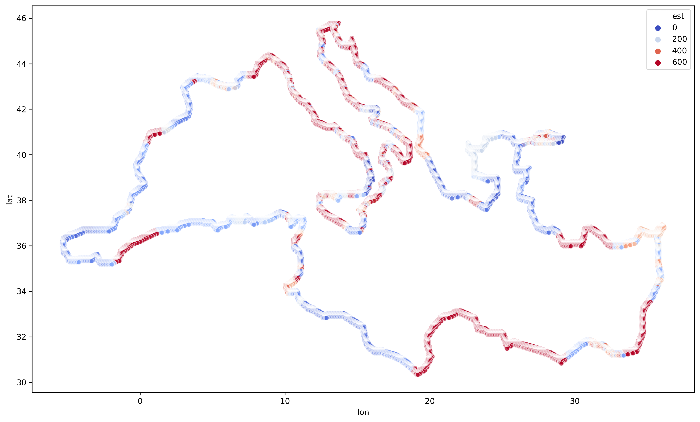
The code is presented in the Listing 6 and output image is presented in the Figure 1.

Listing 6: Scatterplot of HgMe concentrations

# Norm from EPA guidance
epa_norm = 460
hue_norm_custom = (0, epa_norm)

plt.figure(figsize=(12 ,6))
sns.scatterplot(x='lon', y='lat', hue='mea_ug_kg_orig',
                hue_norm=hue_norm_custom,
                palette='coolwarm', alpha=.7,
                data=df)
plt.show()

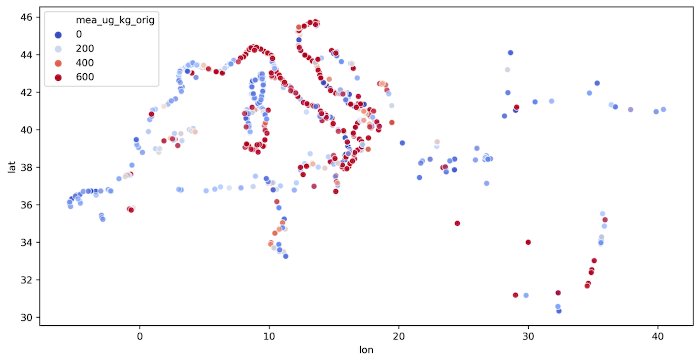
Mercury concentrations near Italy’s coastline exceeds EPA limits and at the same time the largest density of measurements can be seen near the Italy. We shouldn’t conclude anything from it, but it is a good starting point for further analysis.

Shapefile Preparation

We need a canvas to perform interpolation. Or, in other words, a set of points for which we interpolate values. It can be a numpy array, but in our geospatial world, vector files are more useful, and we use shapefile with points along Mediterranean Sea coastline (without borders of isles). File medi_coastline.shp contains prepared points. Let’s read it with Geopandas and look into a spatial DataFrame. Listing 7 is a read operation of a GeoDataFrame object and its coordinate reference system. The main difference between GeoDataFrame and DataFrame is that the first one has additional geometry column and the coordinate reference system (crs) property.

Listing 7: IDW model: read shapefile

gdf = gpd.read_file('medi_coastline.shp')
print(gdf.head())
print(gdf.crs)

Geometry in the gdf is described as the MultiPoint object from shapely package. We can calculate distance between MultiPoint objects and our latitude / longitude pairs of points from the non-spatial DataFrame… but it will make distance calculation more complex. Instead of writing a single complicated function which is transforming MultiPoint into floats, and calculating distance between those points, we are going to create separate function which transform geometry field of GeoDataFrame into latitude / longitude floats. Listing 8 is an example of implementation. Note that we get lat and lon as float point values with the .x and the .y attributes of Point and MultiPoint classes.

Listing 8: IDW model: transform MultiPoint object coordinates into floats

def set_coordinate(point_geometry, coordinate: str):
    """
    Function returns coordinate x or y from multipoint geometry in geodataframe.
    :param point_geometry: MultiPoint or Point geometry,
    :param coordinate: x (longitude) or y (latitude).
    """
    
    if coordinate == 'x':
        try:
            x_coo = point_geometry.x
            return x_coo
        except AttributeError:
            x_coo = point_geometry[0].x
            return x_coo
    elif coordinate == 'y':
        try:
            y_coo = point_geometry.y
            return y_coo
        except AttributeError:
            y_coo = point_geometry[0].y
            return y_coo
    else:
        raise KeyError('Available coordinates: "x" for longitude or "y" for latitude')

gdf['lat'] = gdf['geometry'].apply(set_coordinate, args=('y'))
gdf['lon'] = gdf['geometry'].apply(set_coordinate, args=('x'))
print(gdf.head())

At this moment we have spatial data prepared and we are able to move to the modeling step.

IDW algorithm implementation

Let’s recall IDW equation (1):

$$f(m) = \frac{\sum_{i}\lambda_{i}*f(m_{i})}{\sum_{i}\lambda{i}}; (1)$$

where:

• $f(m)$ is a value at unknown location,
• $i$ is i-th known location,
• $f(m_{i})$ is a value at known location,
• $\lambda$ is a weight assigned to the known location.

We must assign specific weight to get proper results. And weight depends on the distance between known point and unknown point (2).

$$\lambda_{i} = \frac{1}{d_{i}^{p}}; (2)$$

where:

• $d$ is a distance from known point $i$ to the unknown point,
• $p$ is a hyperparameter which controls how strong is a relationship between known point and unknown point. You may set large $p$ if you want to show strong relationship between closest point and very weak influence of distant points. On the other hand, you may set small  $p$ to emphasize fact that points are influencing each other with the same power irrespectively of their distance.

There is a hidden function, because distance $d$ between points must be calculated and the most obvious way to do it is to use Euclidean distance between points:

$$d=\sqrt{(x_{i}-x_{-})^{2}+(y_{i}-y_{-})^{2}}; (3)$$

where $x_{-}$ and $y_{-}$ are coordinates of a point where we want to estimate unknown value.

We have two functions. One is for distance calculation and second is for inverse distance weighting of unknown values. Distance calculation is really simple and we can do it with numpy. Listing 9 is its implementation.

Listing 9: IDW model: distance calculation function

def calculate_distances(all_points, unknown_point):
    # Calculate distances
    d_lat = (all_points[:, 0] - unknown_point[0])**2
    d_lon = (all_points[:, 1] - unknown_point[1])**2
    dists = np.sqrt(d_lon + d_lat)
    return dists

IDW algorithm is a little trickier to implement. We should pass into a function:

• unknown point coordinates (one pair),
• known points’ coordinates and values (multiple pairs),
• power of distance (single value),
• and number of closest distances to the unknown point which are affecting it but this is optional parameter. We may use all available points to estimate value at specific location.

The latter is not included in the equation (1), but it is an optimization for our calculations, and it allows us to control how many neighbors can influence specific point value. It may be very unlikely from the physical perspective that measurements taken near Egyptian coast are correlated with measurements near Croatia, that’s why we are controlling number of neighbors. Figure 3 is a block diagram of IDW algorithm. It seems to be complex algorithm but in reality it is a simple waterfall-style diagram which requires few lines of code (Listing 10).

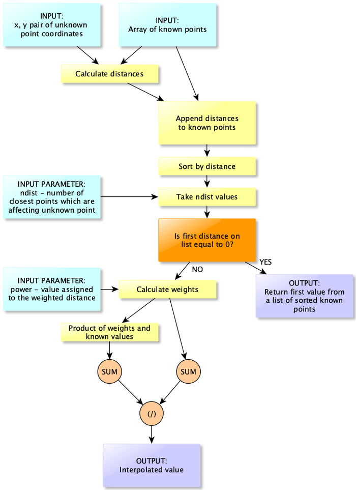
In summary IDW algoirithm works as follow:

1. Calculate distance between point with not-known value and all known points.
2. Append calculated distances as a new column to the numpy array with known distances.
3. Sort this array by the last column.
4. Take ndist number of records for analysis. It may be easily done with numpy indexing.
5. Check if the first distance from a sorted list is equal to 0. If yes, then return point value from this position and end calculations. If no, then calculate weights.
6. Single weight is a ratio of 1 and a distance raised to the n-th power. Calculate weights for each element in the array.
7. Calculate numerator of equation (1). It is a product of weights and known points values.
8. Estimate interpolated point value as a ratio of a sum of all weight-value products and a sum of weights.

Listing 10 is an implementation of this procedure. We are using this function with a GeoDataFrame which we have prepared earlier. We use lambda expression to iterate calculations through all points of the gdf and we set power parameter to 3 and ndist parameter to 4.

Listing 10: IDW model: algorithm implementation

def inverse_distance_weighting(unknown_point, points, power, ndist=10):
    """
    Function estimates values in unknown points with with inverse
    weighted interpolation technique.
    
    INPUT:
    :param unknown_point: lat, lon coordinates of unknown point,
    :param points: (array) list of points [lat, lon, val],
    :param power: (float) constant used to calculate IDW weight
                  -> weight = 1/(distance**power),
    :param ndist: (int) how many closest distances are included
                  in weighting,
    
    OUTPUT:
    :return interpolated_value: (float) interpolated value
                                by IDW method.
    
    Inverse distance weighted interpolation is:
    
    est = SUM(WEIGHTS * KNOWN VALS) / SUM(WEIGHTS)
    and
    WEIGHTS = 1 / (DISTANCE TO UNKNOWN**power)
    
    where:
    power is a constant hyperparameter which tells how much point 
    is influenced by other points. 
    """

    distances = calculate_distances(points, unknown_point)
    points_and_dists = np.c_[points, distances]
    
    # Sort and get only 10 values
    points_and_dists = points_and_dists[points_and_dists[:, -1].argsort()]
    vals_for_idw = points_and_dists[:ndist, :]
    
    # Check if first distance is 0
    if vals_for_idw[0, -1] == 0:
        return vals_for_idw[0, 2]
    else:
        # If its not perform calculations
        weights = 1 / (vals_for_idw[:, -1]**power)
        numerator = weights * vals_for_idw[:, 2]
        interpolated_value = np.sum(numerator) / np.sum(weights)
        return interpolated_value

# Interpolate points

known_points_array = df.to_numpy()
power = 3
nd = 4
gdf['est'] = gdf.apply(lambda col: inverse_distance_weighting(
    [col['lat'], col['lon']],
    known_points_array, power, ndist=nd), axis=1)

Yes, and that’s all! We can now check our interpolated data (Listing 11) and show it as a scatterplot.

Listing 11: IDW model: output visualization

plt.figure(figsize=(15 ,9))
sns.scatterplot(x='lon', y='lat', hue='est', alpha=0.7,
                palette='coolwarm',
                hue_norm=hue_norm_custom, data=gdf)
plt.show()

Final visualization, for the whole coastline of the Mediterranean Sea is presented in the Figure 4. You may see how values are grouped together and create clusters along with some parts of the Mediterranean Sea coastline.

Exercises

1. Use different shapefile for analysis provided here named exercise_points.shp. What do you think about the output?
2. Check what happens when power value is set between 0 and 1, or below 0.
3. Check what happens if you use all points for the estimation.

Next part

>> Three-dimensional interpolation of Mercury Concentrations in the Mediterranean Sea with Python

Bibliography

[1] Health Effects of Exposures to Mercury. United States Environmental Protection Agency. Link: https://www.epa.gov/mercury/health-effects-exposures-mercury

[2] EPA-FDA Fish Advice: Technical Information. United States Environmental Protection Agency. Link: https://www.epa.gov/fish-tech/epa-fda-fish-advice-technical-information

[3] Github with article’s notebooks and shapefiles

[4] Cinnirella, Sergio; Bruno, Delia Evelina; Pirrone, Nicola; Horvat, Milena; Živković, Igor; Evers, David; Johnson, Sarah; Sunderland, Elsie (2019): Mercury concentrations in biota in the Mediterranean Sea, a compilation of 40 years of surveys. PANGAEA, https://doi.org/10.1594/PANGAEA.899723

Changelog

• 2021-07-18: Update of the link to the next lesson.
• 2021-05-21: First release of the article.