Spatial Interpolation 101: Introduction to Inverse Distance Weighting Interpolation Technique
Do you think that points on a map are not enough to tell your story? Me too. Year ago, I’d prepared a presentation for GIS conference and I’d had a point map of measurements. “It won’t be visible” – I thought – “I must do something with it”. Then I spent half the night before presentation on the problem how to interpolate values in locations where measurements were not taken. I’ve used kriging for it, but nowadays I rather focus on simpler approach. This is the Inverse Distance Weighting interpolation technique.
The First Law of Geography
Do you know the first law of geography proposed by Tobler? If not, here it is:
Everything is related to everything else, but near things are more related than distant things.
W.Tobler
What does it mean in practice?
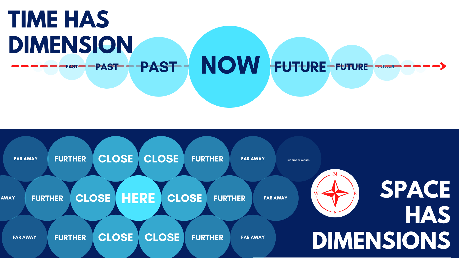
- Temperature in your city is similar to temperature in neighboring city, but it is probably very different than temperature in the city 1000 km South (spatial distance);
- Mean humidity tomorrow will be similar to mean humidity today, but it’ll be different than mean humidity month ago (temporal distance);
- Your closest friends have similar interests and worldview as you, but friends of your friends are dedicated to other things than geostatistics and geography (social distance).
We stick to the spatial distance case and skip other distances, but it is nice to see common ground between different dimensions of our reality. Ok, time to think physics and build our inverse distance weighted interpolation (IDW) model. We have one BIG assumption. That every point is a weighted sum of all other points’ values. What does it mean? We’re going through a specific story to uncover IDW.
The story of shared mood and crocs
IDW concept may be described in two sentences:
- To get value at unseen location you weight values of known locations and sum them.
- Weighting is a function of distance to the unseen location.
That’s it! But still it is hard to understand underlying concept. Thus we will start from the IDW equation (1) and then move to the specific application of IDW to understand its power.
$$f(m) = \frac{\sum_{i}\lambda_{i}*f(m_{i})}{\sum_{i}\lambda{i}}; (1)$$
where:
- $f(m)$ is a value at unknown location,
- $i$ is i-th known location,
- $f(m_{i})$ is a value at known location,
- $\lambda$ is a weight assigned to the known location.
We must assign specific weight to get proper results. And weight depends on the distance between known point and unknown point (2).
$$\lambda_{i} = \frac{1}{d_{i}^{p}}; (2)$$
where:
- $d$ is a distance from known point $i$ to the unknown point,
- $p$ is a hyperparameter which controls how strong is a relationship between known point and unknown point. You may set large $p$ if you want to show strong relationship between closest point and very weak influence of distant points. On the other hand, you may set small $p$ to emphasize fact that points are influencing each other with the same power irrespectively of their distance.
Specific example helps to better understand how lambda parameter affects our analysis. Let’s imagine that you are living in flatland. This land is very strange because your mood is proportional to the mood of your neighbors. Proportion of it may be controlled by some super-three-dimensional entity which changes parameter $p$ of your universe. Larger $p$ increases effective distance between you and your neighbors; their mood is transferred by the valley full of mood-crocs which are eating it. Larger $p$ literally increases number of mood-crocs per each mood route, and if route is longer then more mood-crocs may fit into it (look into the Figures 1-3 if you feel lost here). What happens when $p$ is set to zero (0), one (1) and (2)? We analyze it and with this example you hopefully understand how IDW works.
Set p to 0
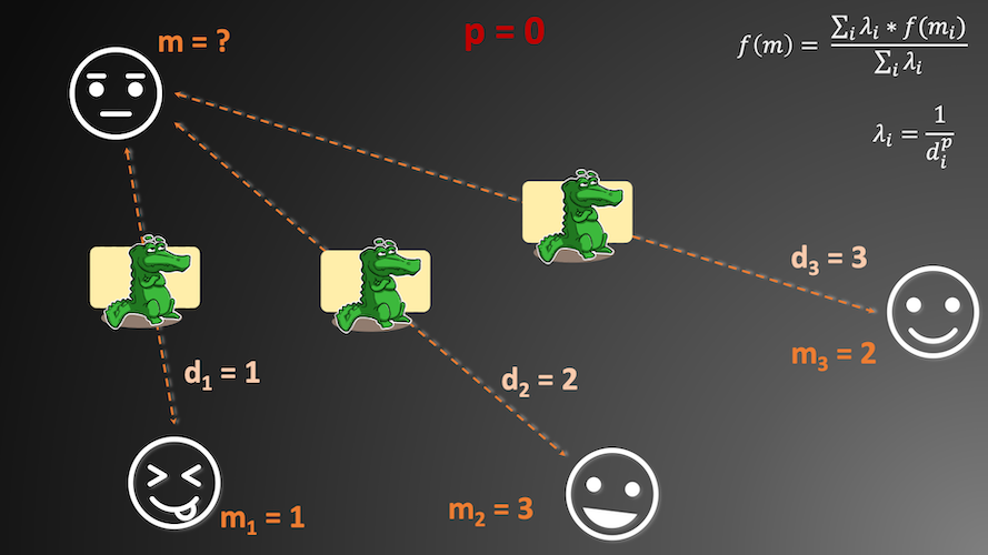
Figure 1 shows three known flatmen with their moods. We have distance between them and the unknown flatman too. In the first step we calculate how many mood-crocs are placed between missing value $m$ and known values $m_{1}$, $m_{2}$ and $m_{3}$ per each mood-transfer route. Those crocs represent weights assigned to the known values; and you may place more crocs (smaller weight, we lost a lot of information on a larger distance) if distance is long. Our distance for every route is different, but if we assume that weighting factor is equal to 0 then our weight (number of crocs) is always one. You should remember from the school algebra that every value raised to 0 gives 1. Weight is always 1 – we set one mood-croc (denominator in $\lambda_{i}$) for every distance. Mood of flatman m is simple average of the other moods and it is equal to 2.
Set p to 1
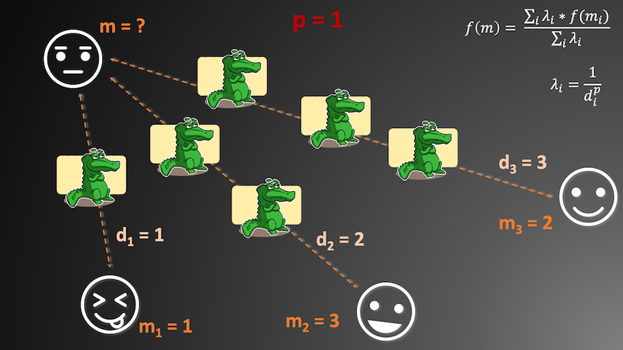
Scenario in Figure 2 is more complicated. We have multiple mood-crocs here because we have set $p$ parameter. As you remember from school algebra, if we raise number to the power of 1 then we get the same number. That’s why number of mood-crocs (weights assigned to each distance) is an inverse proportion of the distance itself. This time we get weighted average of moods in the form:
$$\frac{(1*1+\frac{1}{2}*3+\frac{1}{3}*2)}{(1+\frac{1}{2}+\frac{1}{3})}=\frac{(1+1.5+0.67)}{1.83}=1.73; (3)$$
Set p to 2
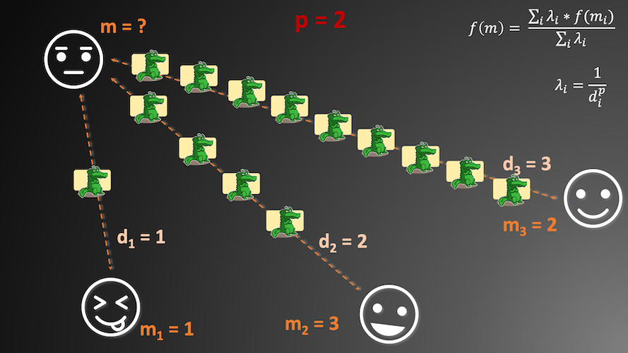
Now interesting story begins. Number of mood-crocs is expanding with the power assigned to the distance. What is the mood of the unknown flatman?
$$\frac{(1*1+\frac{1}{4}*3+\frac{1}{9}*2)}{(1+\frac{1}{4}+\frac{1}{9})}=\frac{(1+0.75+0.22)}{1.36}=1.45; (4)$$
Do you see how power affects effective mood-transfer? Lower mood value is closer to the unknown point, but it still has greatest impact on the final value. And other moods impact decreases quickly with rising power. It is especially visible if you look into the middle part of equation (3) and equation (4). The conclusion is simple: if you want to emphasize close-neighbors interaction then set power to the larger number. But if points in your research area probably interact at a large distance then set power to the small value.
Exercises
- Think of one example of measurements where observations are spatially correlated.
- Why should we care about spatial interpolation?
- What will happen if power is set to the value between 0 and 1? What will happen if power is negative?
Next lesson:
>> Prediction of mercury concentrations in Mediterranean Sea with IDW in Python
Changelog
- 2021-07-18: Update of the link to the next lesson.