Geostatistics: Theoretical Variogram Models

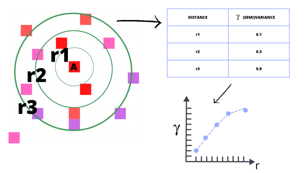
Kriging is a technique of spatial interpolation that uses the dissimilarity measure between observations to interpolate values at missing locations. This “dissimilarity measure” is a semivariogram. And semivariogram is a mathematical function, or more visually, a curve that shows how dissimilar (variance) are points with each other with the rising distance. The Image represents this concept:

Semivariogram has three basic properties:

• nugget: the initial value at a zero distance, in most cases, it is zero, but sometimes it represents a bias in observations.
• sill: the point where semivariogram flattens and reaches approximately 95% of dissimilarity. Sometimes we cannot find a sill; for example, if differences grow exponentially,
• range: is a distance where a variogram reaches its sill. Larger distances are negligible for interpolation.

The crucial step performed by a geostatistican is to choose a valid variogram model for interpolation. The most important are initial distances, before the variogram reaches its sill. That’s why it is good to inspect all available models visually. In this article, we will take a look into different kinds of theoretical models used to analysis of a quasi-random surface generated with a logistic map and blurred with a mean filter:

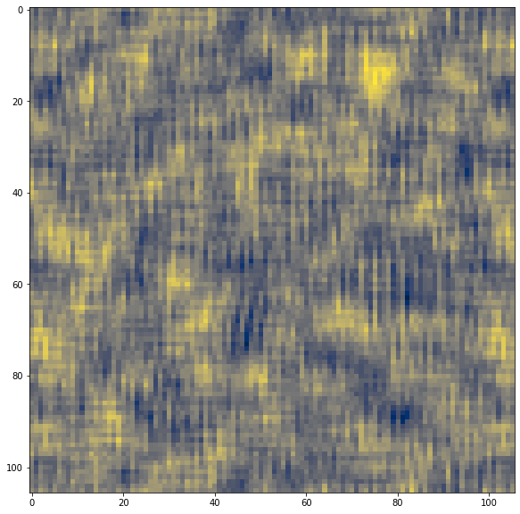
This surface has some large-scale patterns and noise. For the analysis purpose, we will take a look into the omnidirectional variogram of this dataset:

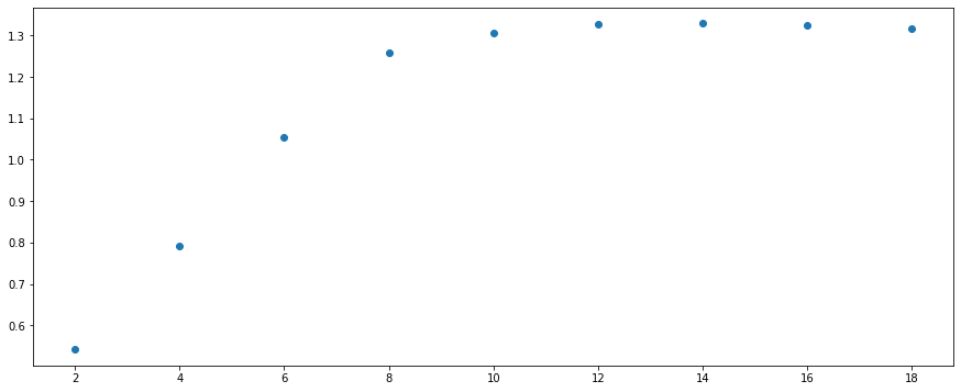
The range and sill of the variogram are not random. The surface was blurred with a mean filter of size 7×7, and we see here that the similarity is close to 7 units of distance. Based on it, we can set properties for a theoretical variogram for:

• nugget: 0
• sill: 1.3
• range: 7

Now, we can take a look at different theoretical models. All models were generated with the Pyinterpolate package.

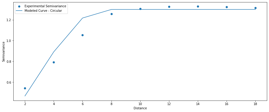
Circular Model

(1) $\gamma = c0 + c[1 – (\frac{2}{\pi} * arccos(\frac{a}{h})) + (\frac{2}{\pi} * \frac{a}{h}) * \sqrt{1 – (\frac{a}{h})^{2}}]$, $0 < a <= h$;

(2) $\gamma = c0 + c$, $a > h$;

(3) $\gamma = 0$, $a = 0$.

where:

• $\gamma$ – semivariance,
• $c0$ – nugget,
• $c$ – sill,
• $a$ – lag,
• $h$ – range.

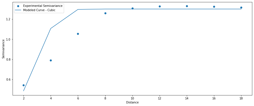
Cubic Model

(1) $\gamma = c0 + c * (7 * (\frac{a}{h})^{2} – 8.75 * (\frac{a}{h})^{3} + 3.5 * (\frac{a}{h})^{5} – 0.75 * (\frac{a}{h})^{7})$, $0 < a <= h$;

(2) $\gamma = c0 + c$, $a > h$;

(3) $\gamma = 0$, $a = 0$.

where:

• $\gamma$ – semivariance,
• $c0$ – nugget,
• $c$ – sill,
• $a$ – lag,
• $h$ – range.

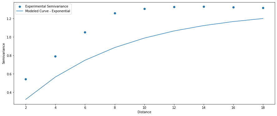
Exponential Model

(1) $\gamma = c0 + c * (1 – \exp({-\frac{a}{h}}))$, $a > 0$,

(2) $\gamma = 0$, $a = 0$.

where:

• $\gamma$ – semivariance,
• $c0$ – nugget,
• $c$ – sill,
• $a$ – lag,
• $h$ – range.

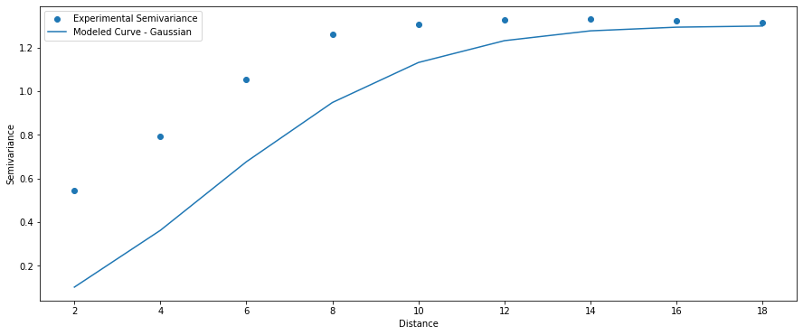
Gaussian Model

(1) $\gamma = c0 + c * (1 – \exp(-\frac{a^{2}}{h^{2}}))$, $a > 0$

(2) $\gamma = 0$, $a = 0$.

where:

• $\gamma$ – semivariance,
• $c0$ – nugget,
• $c$ – sill,
• $a$ – lag,
• $h$ – range.

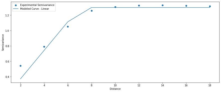
Linear Model

(1) $\gamma = c0 + c * \frac{a}{h}$, $0 < a <= h$;

(2) $\gamma = c0 + c$, $a > h$;

(3) $\gamma = 0$, $a = 0$.

where:

• $\gamma$ – semivariance,
• $c0$ – nugget,
• $c$ – sill,
• $a$ – lag,
• $h$ – range.

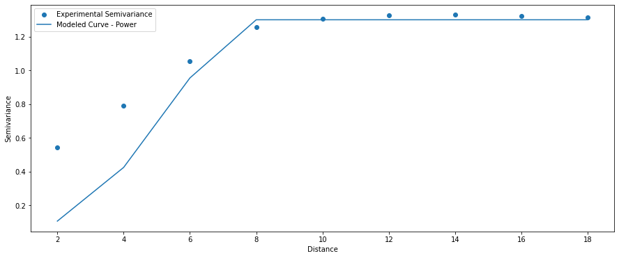
Power Model

(1) $\gamma = c0 + c * (\frac{a}{h})^{2}$, $0 < a <= h$;

(2) $\gamma = c0 + c$, $a > h$;

(3) $\gamma = 0$, $a = 0$.

where:

• $\gamma$ – semivariance,
• $c0$ – nugget,
• $c$ – sill,
• $a$ – lag,
• $h$ – range.

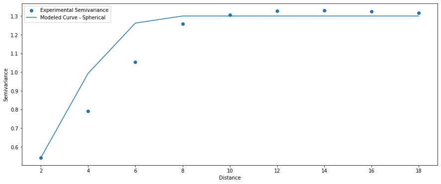
Spherical Model

(1) $\gamma = c0 + c * ( \frac{3}{2} * \frac{a}{h} – 0.5 * (\frac{a}{h})^{3} )$, $0 < a <= h$;

(2) $\gamma = c0 + c$, $a > h$;

(3) $\gamma = 0$, $a = 0$.

where:

• $\gamma$ – semivariance,
• $c0$ – nugget,
• $c$ – sill,
• $a$ – lag,
• $h$ – range.

Comparison of multiple models

The best idea is to compare multiple models with the experimental points:

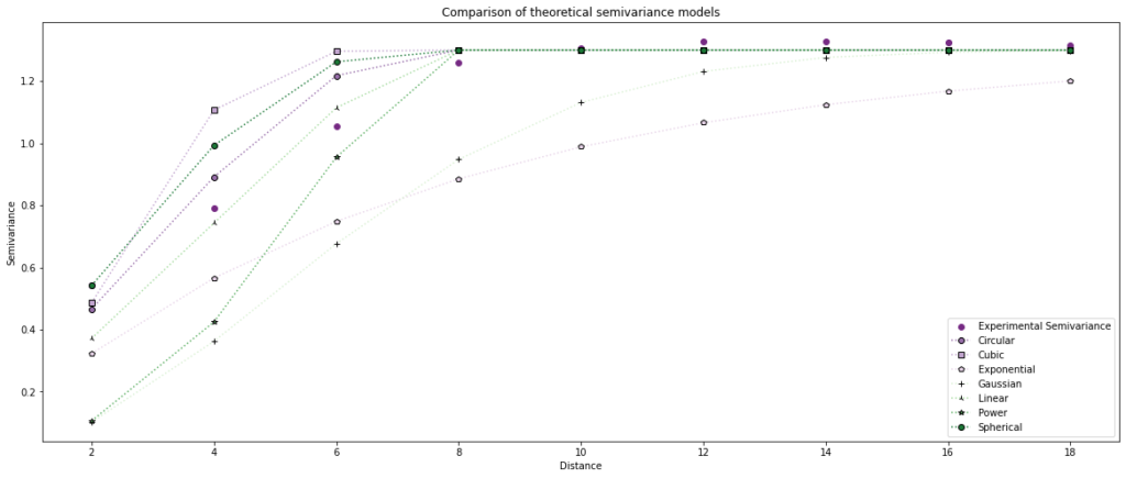
This comparison clearly shows that the linear and circular models are the best in our case. We should be aware that “automatic fitting” of the best model may return a model that best fits long-distance (semi)variances (for example, lags 10-18) and works poorly for short-range values. It is a huuuge mistake! We should always minimize the error of the first few lags because those distances are most similar, and they describe a correlation between points!

Bibliography

Want to learn more? Use those resources:

• Webster, R., Oliver, M.A. Geostatistics for environmental scientist (2nd ed.). ISBN: 978-0-470-02858-2. Wiley 2007.
• Oliver, M.A., Webster, R. Basic steps in geostatistics: the variogram and Kriging. ISBN: 978-3-319-15865-5. Springer 2015.
• Armstrong, M. Basic Linear Geostatistics. ISBN: 978-3-642-58727-6. Springer 1998.
• McBratney, A. B., Webster R. Choosing Functions for Semivariograms of Soil Properties and Fitting Them to Sampling Estimates. Journal of Soil Science 37: 617–639. 1986.
• Moliński, S., (2022). Pyinterpolate: Spatial interpolation in Python for point measurements and aggregated datasets. Journal of Open Source Software, 7(70), 2869, https://doi.org/10.21105/joss.02869

Want to experiment by yourself? Use this package:

• https://pypi.org/project/pyinterpolate/