Data Engineering: The Test Coverage for the Scientific Software

Decorative image with two ants on a grass leaf.

Data Engineering: The Test Coverage for the Scientific Software

September 5, 2021

Data Engineering, Pyinterpolate, Python, R&D, Testing

In this tutorial, we will learn about the different types of tests that could cover the scientific package. We are going to create unit and functional tests for the code developed within the Pyinterpolate package. We see how to use Jupyter Notebooks and additional tutorial files for testing.

Introduction

Whenever code is changed or a new feature is added we should perform tests to ensure that everything works as it should be. We have few different levels of test to perform. The list below represents all steps within the Pyinterpolate package required to be sure that everything works (hopefully) fine.

Write unit tests in test directory of the package to check if input data structure is valid or if returned values are within specific range or are of specific type. Use unittests package. Group tests in regards to the module within you’re working. As example if you implement new Kriging technique put your tests inside test.kriging module. Name your test file with a prefix test_ and follow unittest naming conventions of functions and classes.
Write a logical test where you know exactly what should be returned. This step is very important in the development of scientific software so pen & paper are equally important as keybord & monitor. Where it’s possible use examples from the literature and try to achieve the same results with the same inputs. If this is not possible justify why function is usable and why your results are different than those in the literature.
Run all tests within the test package. You have two main options: use PyCharm or Python console.
Update all tutorials where the feature change or the new development may affect process or write the new tutorial with the new feature usage included.

To make things easier to understand we will go through the example of calculate_seimvariance() function from the Pyinterpolate and we will uncover the points above in greater detail.

Example Function

To start with the development we must first do two things:

Write an equation or create block diagram algorithm of the function,
Prepare dataset for logic tests.

Those two steps prepare our mental model. In the ideal situation, we should have the mathematical equation or algorithm blocks and a sample dataset from publications. Fortunately for us, the experimental semivariogram calculation process is well described in the book Basic Linear Geostatistics written by Margaret Armstrong in 1998 (pages 47-52 for this tutorial). (If you’re a geostatistican and you haven’t read this book yet then do it as soon as you can. This resource is a gem among books for geostatistics and Pyinterpolate relies heavily on it).

Let’s start from the equation for experimental semivariogram:

$$\gamma'(h) = \frac{1}{2 * N(h)} \sum_{i=1}^{N(h)} [Z(x_{i} + h) – Z(x_{i})]^2$$

where $\gamma'(h)$ is a semivariance for a given lag $h$, $x_{i}$ are the locations of samples, $Z(x_{i})$ are their values and $N(h)$ is the number of pairs $(x_{i}, x_{i + h})$. What does it mean in practice? We may freely translate it to the sentence that semivariance at a given interval of distances is a halved mean squared error of all points pairs that are in a given interval. Based on this assumption we can prepare the first draft of our algorithm as a set of steps to do:

(1) Read Data as an array of triplets x, y, value,
(2) Calculate distances between each element from the array,
(3) Create lags list to group semivariances (lags are separation distances $h$),
(4a) For each lag group calculated distances to select points within a specific range (lag),
(4b) Calculated mean squared error between all points pairs and divide it by two (each pair is taken twice a time),
(4c) Store calculated semivariance along the lag and number of points used for calculation within array lag, semivariance, number of points,
(5) Return array of lags and their semivariances.

After this step, we should probably see some limits and dependencies within the algorithm output. We are ready to implement unit tests.

Unit Tests

We will create a simple unit test that checks if all results are positive. (Lags can be only positive because distances are not negative. The semivariance is positive too, since it is a squared difference it must always be a positive number). First, let’s create a Python file within the test.semivariance module. All files with unit tests should have a prefix test_. That’s why we name our file test_calculate_semivariance and a full path to the file should be:

pyinterpolate/test/semivariance/test_calculate_semivariance.py

In the beginning, we must import calculate_semivariance() method and unittest module.

import unittest
from pyinterpolate.semivariance import calculate_semivariance

To write a test we must create a Python class that starts with a Test_ prefix. Usually, it is named TestYourFunctionOrModuleName, in our case: TestCalculateSemivariance. This class inherits from the unittest.TestCase. We can skip the explanation of what inheritance is. The key is to understand that we can use methods from unittest.TestCase in our class TestCalculateSemivariance and those methods allow us to write unit tests. Let’s update our script with this new piece of information:

import unittest
from pyinterpolate.semivariance import calculate_semivariance

class TestCalculateSemivariance(unittest.TestCase):

	def test_calculate_semivariance(self):
		pass

The good practice with unit testing is to have data that is not dependent on external sources or processes. In other words, we use mostly static files with known datasets or artificial arrays. Those arrays may be filled with random numbers of specific distribution or hard-coded values which are simulating possible input. We are going to create one array for the sake of simplicity:

INPUT = [8, 6, 4, 3, 6, 5, 7, 2, 8, 9, 5, 6, 3]

This array is not random. It comes from the Basic Linear Geostatistic and it is presented on page 48 of this book. It has an important property: it is so simple that we can calculate semivariance by hand… and it will be a topic of functional testing scenario. Now we consider the output test to check if all outputs are positive numbers. Function calculate_semivariance() returns list of triplets: [lag, semivariance, number of point pairs] and we must check them all. First, calculate semivariances up to lag 5 by hand.

Lag 0

$$\gamma(h_{0})= 0$$

The expected output: [0, 0, 13]

Lag 1

$$\gamma(h_{1})=\frac{1}{224}2(4+4+1+9+1+4+25+36+1+16+1+9)=\frac{111}{24}=4.625$$

The expected output: [1, 4.625, 24]

Lag 2

$$\gamma(h_{2})= \frac{1}{222}2(16+9+4+4+1+9+1+49+9+9+4)=\frac{115}{22}=5.227$$

The expected output: [2, 5.227, 22]

Lag 3

$$\gamma(h_{3})= \frac{1}{220}2(25+0+1+16+16+9+4+9+4+36)=\frac{120}{20}=6.0$$

The expected output: [3, 6.0, 20]

Lag 4

$$\gamma(h_{4})= \frac{1}{218}2(4+1+9+1+4+16+4+16+25)=\frac{80}{18}=4.444$$

The expected output: [4, 4.444, 18]

Lag 5

$$\gamma(h_{5})= \frac{1}{216}2(9+1+4+25+9+0+1+1)=\frac{50}{16}=3.125$$

The expected output: [5, 5.0, 16]

We prepare a static (constant) variable with the expected output values. At this step, we import NumPy to create an output of the same type as the output returned by the calculate_semivariance() function.

import unittest
from pyinterpolate.semivariance import calculate_semivariance

class TestCalculateSemivariance(unittest.TestCase):

	def test_calculate_semivariance(self):
		INPUT = [8, 6, 4, 3, 6, 5, 7, 2, 8, 9, 5, 6, 3]
		EXPECTED_OUTPUT = np.array([
			[0, 0, 13],
			[1, 4.625, 24],
			[2, 5.227, 22],
			[3, 6.0, 20],
			[4, 4.444, 18],
			[5, 3.125, 16]
		])

The first test is very simple: we should check if the output values from the function are positive. The thing is easy because each column from the output array MUST BE a positive number but we are going to focus only on the middle column with the experimental semivariance values. So let’s begin testing! Tests in Python are written with the assert keyword. We use specific conditions with this keyword, for example, we can:

check if values are equal,
check if values are not equal,
check if given value is True or False,
check if function raises specific error,
and more… described here.

For this tutorial, we will perform a simple test to check if all values of the output are greater than zero. Unittest package has method assertGreaterEqual(a, b) which can be used to test this case but we rather will use assertTrue() to test if every compared record in the array is greater than 0, or it is True. How are we going to test it? NumPy has a great system of checking different conditions on arrays. We can test any condition with the syntax:

boolean_test = my_array[my_array >= 0]

Variable boolean_test is an array of the same size as my_array but with True and False values at the specific positions where the condition has been met or hasn’t. We can add a method .all() to check if every value in the boolean array is True:

boolean_test = my_array[my_array >= 0]
boolean_output = boolean_test.all()

Then we can assert value to our test. In this case, let’s start with the artificial array EXPECTED_OUTPUT. Even if we know that everything is ok we should test the output to be sure that the test is designed properly:

import unittest
from pyinterpolate.semivariance import calculate_semivariance

class TestCalculateSemivariance(unittest.TestCase):

	def test_calculate_semivariance(self):
		INPUT = [8, 6, 4, 3, 6, 5, 7, 2, 8, 9, 5, 6, 3]
		EXPECTED_OUTPUT = np.array([
			[0, 0, 13],
			[1, 4.625, 24],
			[2, 5.227, 22],
			[3, 6.0, 20],
			[4, 4.444, 18],
			[5, 3.125, 16]
		])
		expected_output_values = EXPECTED_OUTPUT[:, 1].copy()
		
		boolean_test = (expected_output_values >= 0).all()
		
		assertTrue(boolean_test, 'Test failed. Calculated values are below zero which is non-physical. Check your data.')

The test should definitively pass but you may want to check what’ll happen if you change one value to the negative number:

import unittest
from pyinterpolate.semivariance import calculate_semivariance

class TestCalculateSemivariance(unittest.TestCase):

	def test_calculate_semivariance(self):
		INPUT = [8, 6, 4, 3, 6, 5, 7, 2, 8, 9, 5, 6, 3]
		EXPECTED_OUTPUT = np.array([
			[0, 0, 13],
			[1, 4.625, 24],
			[2, 5.227, 22],
			[3, -6.0, 20],
			[4, 4.444, 18],
			[5, 3.125, 16]
		])
		expected_output_values = EXPECTED_OUTPUT[:, 1].copy()
		
		boolean_test = (expected_output_values >= 0).all()
		
		self.assertTrue(boolean_test, 'Test failed. Calculated values are below zero which is non-physical. Check your data.')

Surprised!? We got the assertion error and it informs us that we haven’t correctly implemented something. Let’s remove the minus sign from the expected output lag’s number 3 semivariance and test the baseline function, but leave the EXPECTED_OUTPUT variable without a test.

Function calculate_semivariance(data, step_size, max_range) has three parameters. From the documentation we know that:

data parameter is numpy array of coordinates and their values,
step_size parameter is a distance between lags and has a float type,
max_range is a maximum range of analysis and has a float type.

From this description, we see that our INPUT variable is not what’s expected by the algorithm. We will change it and we set step_size and max_range parameters within our test case and we remove EXPECTED_OUTPUT variable because for this concrete test we do not need it. We change the name of the unit test to the test_positive_output(self) to make our test goal clear.

import unittest
from pyinterpolate.semivariance import calculate_semivariance

class TestCalculateSemivariance(unittest.TestCase):

	def test_positive_output(self):
		INPUT = np.array([
			[0, 0, 8],
			[1, 0, 6],
			[2, 0, 4], 
			[3, 0, 3], 
			[4, 0, 6], 
			[5, 0, 5], 
			[6, 0, 7], 
			[7, 0, 2], 
			[8, 0, 8], 
			[9, 0, 9], 
			[10, 0, 5], 
			[11, 0, 6], 
			[12, 0, 3]
		])
		
		# Calculate experimental semivariance
		t_step_size = 1.1
		t_max_range = 6
		
		experimental_semivariance = calculate_semivariance(INPUT, t_step_size, t_max_range)
		
		boolean_test = (experimental_semivariance >= 0).all()
		
		self.assertTrue(boolean_test, 'Test failed. Calculated values are below zero which is non-physical.')

Terrific! We’ve performed our first unit test! (By the way: it is implemented in the package).

Logical and functional testing

The next type of testing is a functional test. Do you remember how we’ve calculated semivariance manually in the previous part? We are going to use the EXPECTED_OUTPUT array from the last test:

EXPECTED_OUTPUT = np.array([
			[0, 0, 13],
			[1, 4.625, 24],
			[2, 5.227, 22],
			[3, 6.0, 20],
			[4, 4.444, 18],
			[5, 3.125, 16]
		])

Why do we need it? A unit test is important for software development but scientific software development is even more rigorous! We need to prove that our function works as expected for a wide range of scenarios. It is not an easy task. Some algorithms haven’t be proven mathematically… But we have an advantage: geostatistics is a well-established discipline and we can use external sources and pen and paper for testing.

We’d created a functionality test in the previous example but we didn’t use it. The idea is to create a simple example now, that can test if our program calculates semivariance correctly. We’ve taken an example array from the literature and we calculated semivariance values for few lags by hand. We assume that the results are correct (if you are not sure check records with the book; but I couldn’t assure you that everyone is wrong but your program).

The EXPECTED_OUTPUT array is a static entity against which we can compare the results of our algorithm. We can distinguish few steps which need to be done for the logic test:

Get the reference input and create the reference output. This could be calculated manually, derived from the literature or estimated by the other program which produces the right output.
Store reference output as the script values or as the non-changing file. The key is to never change values in this output throughout the testing flow.
Estimate the expected output from the reference input with your algorithm.
Compare the expected output and the reference output. If both are the same (or very close) then test is passed.

A few steps of functional testing can be very misleading if we consider the complexity of the whole process. There are traps in here, and sometimes it is hard to avoid them:

the reference input covers very unusual scenario, as example it is created from the dataset with the uniform distribution but in reality data follows other types of distribution,
the reference input and output do not exist or the reference data is not publicly available (frequent problem with publications),
it’s hard to calculate the reference output manually.

But the biggest, and the most dangerous problem which sometimes relates to the previous obstacles is the reference output assignation from the developed algorithm itself (we don’t know the reference output and we create it from our algorithm itself…). Is it bad? Yes, it is. Is it sometimes the only (fast and dirty) way of development? Yes, it is. But even in this scenario we usually perform some kind of sanity check against our belief how the output should look like. Let’s put aside the dirty testing and come back to our case. We have the expected output and we have the reference input. With both, we can create the functionality test within our package!

The code will be similar to the unit test, e.g.: there’s the same building logic behind it. We define a function within the class that inherits from unittest.TestCase. Within this function, we define the reference input and the reference output. We run the algorithm on the reference input and compare results to the reference output. Numpy has special assertion methods and we are going to pick asset_almost_equal() for our test scenario. When we compare two arrays with floating-point precision it is better to use this assertion which allows a small difference between the records in the compared arrays. The code itself is presented below:

import unittest
from numpy.testing import assert_almost_equal

from pyinterpolate.semivariance.semivariogram_estimation.calculate_semivariance import calculate_semivariance

class TestCalculateSemivariance(unittest.TestCase):
    """
    HERE COULD BE A THE PART FOR OTHER TESTS
    """
    def test_against_expected_value_1(self):

        REFERENCE_INPUT = np.array([
            [0, 0, 8],
            [1, 0, 6],
            [2, 0, 4],
            [3, 0, 3],
            [4, 0, 6],
            [5, 0, 5],
            [6, 0, 7],
            [7, 0, 2],
            [8, 0, 8],
            [9, 0, 9],
            [10, 0, 5],
            [11, 0, 6],
            [12, 0, 3]
        ])

        EXPECTED_OUTPUT = np.array([
			[0, 0, 13],
			[1, 4.625, 24],
			[2, 5.227, 22],
			[3, 6.0, 20],
			[4, 4.444, 18],
			[5, 3.125, 16]
		])

        # Calculate experimental semivariance
        t_step_size = 1
        t_max_range = 6

        experimental_semivariance = calculate_semivariance(REFERENCE_INPUT, t_step_size, t_max_range)

        # Get first five lags
        estimated_output = experimental_semivariance[:6, :]

        # Compare
        err_msg = 'The reference output and the estimated output are too dissimilar, check your algorithm'
        assert_almost_equal(estimated_output, EXPECTED_OUTPUT, 3, err_msg=err_msg)

This code is coming from the official codebase, you can look there too, to see how it is slightly rearranged within the test script.

How to run unit tests

There are two main ways to perform a unit test: within the IDE or manually, from the terminal. We prefer to use PyCharm for the tests and the next example will show how those can be performed within this IDE.

PyCharm

PyCharm Single test

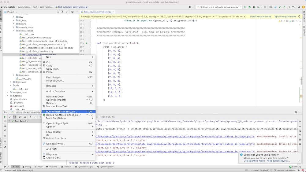
The unit testing with PyCharm is very easy. You should open Project view on the left side. You will see a window with the project tree. Navigate to the specific file with unit tests, click the right mouse button, select Run Unittests in test_case_. A test is under its way. After a while, you will see the test results in the bottom window.

Figure 1: Run Single Unit Test in PyCharm.

PyCharm Multiple tests

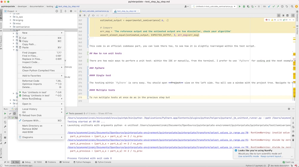
To run multiple tests at once do as in the previous step but right-click on the directory with tests and select Run Unittests in tests. All tests for Pyinterpolate take about a minute to go.

Figure 2: Run Multiple Tests at once in PyCharm.

Console

A test from the console is slightly more complex than from the IDE. It is required to be within a test directory and to have installed all required packages – in the normal scenario those are installed within the virtual environment or the conda environment. Next:

Activate environment with the dependencies of a package.
Navigate to the directory with tests.

The next steps differ in the case if we’d like to test one script or every case in the package.

Console Single test

Navigate to the directory with a specific test.
Run unittest script:

python -m unittest test_calculate_semivariance

Console Multiple tests

Navigate to the parent directory of tests which you want to cover.
Run unittest script:

python -m unittest

Use a Tutorial for Testing

Pyinterpolate follows a specific flow of development. In the beginning, each feature is developed within the Jupyter Notebook. We build a function or class with the concrete example in mind. Then it is easy to transform a development notebook into a tutorial. About half of the tutorials were developed in this manner. The next big thing with the tutorials is that we can perform the so-called sanity check within them. There are bugs, especially logical, which are not covered by the unit tests or functionality testing. Tutorials cover a large part of the workflow and it makes them a great resource for program testing. Thus after the implementation of new features or changes inside old features, we always run all affected tutorials. Probably you saw that each tutorial has a changelog table and there are records related to the feature changes.

The development and testing within notebooks can be summarized in a few steps:

Develop a feature in the notebook. (Development)
Write a tutorial related to this feature. (Development)
After any change in the feature run tutorial to check if everything works fine. (Maintenance and Testing)
After development of the new features test affected tutorials if there are any. (Maintenance and Testing)

We strongly encourage any developer to go within this pattern. It builds confidence about the proposed development and the understanding of the covered topics, as semivariogram modeling, kriging, and so on. Running all tutorials before a major release of Pyinterpolate is mandatory, even if the changes shouldn’t affect a specific tutorial workflow. It is another kind of test and it assures that users get a very good product.

Summary

You have learned how to:

write the unit test,
write and prepare the functionality test,
run tests from the IDE and console,
use tutorials as the playground for tests.

If you are still not sure about anything in this article then write an Issue within the package repository. We will answer all your questions!